Vector quantization (VQ)#
Suppose you have recorded sounds at different locations and want to categorize them into similar groups. In other words, you have a stochastic vector \(x\) which you want to characterize with a simple description. For example, categories could correspond to office, street, hallway and cafeteria. A classic way for this task is to choose template vectors \(c_{k}\), which represents a typical sound in each environment \(k\). To categorize the sounds, you then find that template vector which is closest to your recording \(x\). In mathematical notation, you search for a \(k^{^*}\) by
The above expression thus calculates the squared error between \(x \) and each of the vectors \(c_{k}\) and chooses the index \(k \) of the vector with the smallest error. The vectors \(c_{k}\) then represent a codebook and the vector \(x\) is quantized to \(c_{k^*}\). This is the basic idea behind vector quantization, which is also known as k-means.
A illustration of a simple vector codebook is shown on the right. The input data is a Gaussian distribution shown with grey dots and the codebook vectors \(c_{k}\) with red circles. For each input vector we thus search for the nearest codebook vector and the borders of the regions where input vectors are assigned to a particular codebook vector are illustrated with blue lines. These regions are known as Voronoi regions and the blue lines are the decision-boundaries between codebook vectors.
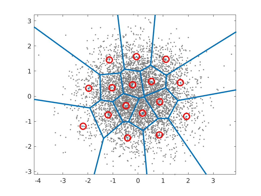
Example of a codebook for a 2D Gaussian with 16 code vectors.
Metric for codebook quality#
Suppose then that you have a large collection of vectors \(x_{h}\), and you want to find out how well this codebook represents the input data. The expectation of the squared error is approximately the mean over your data, such that
where \(E[ ]\) is the expectation operator and \(N\) is the number of input vectors \(x_{h}\). Above, we thus find the codebook vector which is closest to \(x_{h}\), find its squared error and take the expectation over all possible inputs. This is approximately equal to the mean of those squared errors over a set of input vectors.
To find the best set of codebook vectors \(c_{k}\), we then need to minimize the mean squared error as
or more specifically, for a dataset as
Unfortunately we do not have an analytic solution for this optimization problem, but have to use numerical, iterative methods.
Codebook optimization#
Expectation maximization (EM)#
Classical methods for finding the best codebook are derivatives of expectation maximization (EM), which is based on two alternating steps:
Expectation Maximation (EM) algorithm:
For every vector \(x_{h}\) in a large database, find the best codebook vector \(c_{k}\).
For every codebook vector \(c_{k}\);
Find all vectors \(x_{h}\) assigned to that codevector.
Calculate mean of those vectors.
Assign the mean as a new value for the codevector.
If converged then stop, otherwise go to 1.
This algorithm is guaranteed to give a codebook at every step which is not worse than the previous codebook. That is, at each iteration will improve until it finds a local minimum, where it stops changing. The reason is that each step in the iteration finds a partial best-solution. In the first step, we find the best matching codebook vectors for each data vectors \(x_{h}\). In the second step, we find the within-category mean. That is, the new mean is more accurate than the previous codevector in that it reduces the average squared error. If the mean is equal to the previous codevector, then there is no improvement.
As noted above, this algorithm is the basis to most vector quantization codebook optimization algorithms. There are a multiple reasons why this simple algorithm is usually not sufficient alone. Most importantly, the above algorithm is slow to converge to a stable solution and it often finds a local minimum instead of a global minimum.
To improve performance, we can apply several heuristic approaches. For example, we can start with a small codebook \( \{ c_k \}_{k=1}^K \) of \(K\) elements and optimize it with the EM algorithm. We then split the codebook into two, offset by a small delta \(d\), such that \( \|d\|<\epsilon \) and make the new codebook \( \{ \hat c_k \}_{k=1}^{2K} := \{ c_k,\, c_k+d \}_{k=1}^K \) of 2\(K\) elements. We then rerun the EM algorithm on the new codebook. The codebook thus doubles in size at every iteration and we continue until we have the desired codebook size.
The advantage of this approach is that it focuses attention to the big bulk of datapoints \(x_{k}\), and ignores outliers. The outcome is then expected to be more stable and the likelihood of converging to a local minimum is smaller. The downside is that with this approach it is then more difficult to find small separated islands. That is, because the initial codebook is near the center of the whole mass of datapoints, adding a small delta to the codebook vectors keeps the new codevectors near the center-of-mass.
Conversely, we can start with a large codebook, say treat the whole input database \(x_{k}\) as a codebook. We can then iteratively merge pairs of points which are close to each other, until the codebook is reduced to the desired size. Needless to say, this will be a slow process if the database is large, but will be very efficient in finding separated islands of points.
In any case, optimization of vector codebooks is a difficult task and we have no practical algorithms which would be guaranteed to find the global optimum. Like in many other machine learning problems, optimizing the codebook is very much about learning to know your data. You should first use one algorithm and then analyse the output to find out what can be improved, and keep repeating this optimization and analyse process until the output is sufficiently good.
Optimization with machine learning platforms#
A modern approach to modelling is machine learning, where complex phenomena are modelled with neural networks. Typically they are trained with gradient-descent type methods, where parameters are iteratively nudged towards the minimum, by following the steepest gradient. Since such gradients can be automatically derived on machine learning platforms (using the chain rule), they can be applied on very complex models. Consequently, they have become very popular and succesful.
The same type of training can be readily applied to vector quantizers as well. However, there is a practical problem with this approach. Estimation of the gradients of the parameters with the chain-rule requires that all intermediate gradients are non-zero. Quantizers are however piece-wise constant such that their gradients are uniformly zero, thus disabling the chain rule and gradient descent for all parameters which lie behind the quantizer in the computational graph. A practical solution is known as pass-through, where gradients are passed unchanged through the quantizer. This approximation is simple to implement and provides often adequate performance.
While this approach converges slower than the EM-algorithm, it is often beneficial since it allows optimization of an entire system to a single goal. That is, if we have several modules in a system, it is beneficial if their joint interaction is taken into account in the optimization. If modules are optimized independently, it is difficult to anticpate all interactions and the system performance can remain far from optimal.
Algorithmic complexity#
Vector quantization is manageable for relatively small codebooks of, say, \(K=32\) codevectors. That corresponds to 5 bits of information. For many applications, that does not give sufficient accuracy - the mean squared error is too large. For example, the linear predictive models in speech coding could be quantized with 30 bits, which corresponds to \( K=2^{30}\approx 10^9 \) codevectors. To find the best codevector for a vector \(x\) of length \(N=16\), we would then need to calculate the distance between every codebook vector and \(x\), which amounts to approximately \( 16\times10^9= 1.6\times10^{10} \) operations. That is infeasible in on-line applications on mobile devices. Instead, we need to find a simpler method which retains the best aspects of the algorithm, but reduces algorithmic complexity.
A heuristic approach is to use successive codebooks, where at each iteration, we quantize the error of the last iteration. That is, let’s say that on the first iteration we have 8 bits, corresponding to a codebook \(c_{k}\) of \(K=256\) vectors. We find the best matching codevector \(c_{k^*}\) and calculate the residual \( x':=x-c_{k^*} \) . In the second stage, we would then find the best matching vector for \(x'\) from a second codebook \(c_{k}'\). We can add as many layers of codebooks as we want until the desired number of bits has been consumed. This approach is known as a multi-stage vector quantizer.
Where ordinary vector quantization can find the optimal solution, split vector quantization generally does not give a global optimum. It does give good solutions, though, but with an algorithmic complexity which very much lower than ordinary vector quantization. For example, in the above example of 30 bits, we could assign three consecutive layers of codebooks with 10 bits / \(K=1024\) each, such that the overall complexity is \( 3\times 16\times 2^{10} \approx 5\times10^4, \) which gives an improvement with a factor of \( 3.5\times10^5. \) Given that the reduction in accuracy is manageable, this is a major improvement in complexity.
Applications#
Probably the most important application where vector quantization is used in speech processing, is speech coding with Code-excited linear prediction (CELP), where
linear predictive coefficients (LPC) are transformed to line spectral frequencies (LSFs), which are often encoded with multi-stage vector quantizers.
gains (signal energy) of the residual and long term prediction are jointly encoded with a single stage vector quantizer.
Other typical applications include
In optimization of Gaussian mixture models (GMMs), it is useful to use vector quantization to find a first-guess of the means of each mixture.
Discussion#
The benefit of vector quantization is that it is a simple algorithm which gives high accuracy. In fact, for quantizing complicated data, vector quantization is (in theory) optimal in fixed-rate coding applications. It is simple in the sense that an experienced engineer can implement it in a matter of hours. Downsides with vector quantization include
Complexity; for accurate quantization you need prohibitively large codebooks. The method therefore does not scale up nicely to big problems.
Difficult optimization;
Training data; The amount of data needed to optimize a vector codebook is large. Each codebook vector must be assigned to a large number of data vectors, such that calculation of the mean (in the EM algorithm) is meaningful.
Convergence; we have no assurance that optimization algorithms find the global optimum and we have no assurance that local minima are “good enough”.
Lack of flexibility; the codebook has a fixed size. If we would like to use codebooks of different sizes, for example, if we want to transmit data with a variable bit-rate, then we have to optimize and store a large codebook for every possible bitrate.
Blindness to inherent structures; this model describes data with a codebook, without any deeper understanding of what the data looks like within each category. For example, say we have two classes, speech and non-speech. Even if speech is very flexible, the non-speech class is much, much larger. Speech is a very small subset of all possible sounds. Therefore, the within-class variance will be much larger in the non-speech class. Consequently, the accuracy in the non-speech class would be much lower.
As a consequence, we would be tempted to increase the number of codevectors such that we get uniform accuracy in both classes. But then we loose the correspondence between codevectors and natural descriptions of the signal.