8.1. Voice Activity Detection (VAD)

8.1.1. Introduction

• Voice activity detection (VAD) (or speech activity detection, or speech detection) refers to a class of methods which detect whether a sound signal contains speech or not.

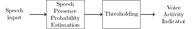
• A closely related and partly overlapping task is speech presence probability (SPP) estimation.

  • Instead of a binary present/not-present decision, SPP gives a probability level that the signal contains speech.

  • A VAD can be derived from SPP by setting a threshold probability above which the signal is considered to contain speech.

  • In most cases, SPP is thus the more fundamental problem.

• Voice activity detection is used as a pre-processing algorithm for almost all other speech processing methods.

  • In speech coding, it is used to to determine when speech transmission can be switched off to reduce the amount of transmitted data.

  • In speech recognition, it is used to find out what parts of the signal should be fed to the recognition engine. Since recognition is a computationally complex operation, ignoring non-speech parts saves CPU power.

• VAD or SPP is thus used mostly as a resource-saving operation.

• In speech enhancement, where we want to reduce or remove noise in a speech signal, we can estimate noise characteristics from non-speech parts (learn/adapt) and remove noise from the speech parts (apply).

• A closely related method in audio applications is noise gateing, where typically a microphone signal is muted whenever there is no signal present.

  • For example, when a singer is not singing in the microphone, then the microphone is off. When the singer is not singing, microphone signal is only noise and therefore the noise gate removes (gates) noise.

• VADs can thus also be used in improving signal quality.

8.1.2. Low-noise VAD = Trivial case

• To introduce basic vocabulary and methodology, let us consider a case where a speaker is speaking in an (otherwise) silent environment.

  • When there is no speech, there is silence.

  • (Any) Signal activity indicates voice activity.

• Signal activity can be measured by, for example, estimating signal energy per frame \(\Rightarrow\) the energy thresholding algorithm.

Show code cell source Hide code cell source

# Initialization for all
from scipy.io import wavfile
import numpy as np 
import matplotlib.pyplot as plt
import IPython.display as ipd 
import scipy 
import scipy.fft 

#from helper_functions import stft, istft, halfsinewindow

Show code cell source Hide code cell source

def stft(data,fs,window_length_ms=30,window_step_ms=20,windowing_function=None):
    window_length = int(window_length_ms*fs/2000)*2
    window_step = int(window_step_ms*fs/1000)
    if windowing_function is None:
        windowing_function = np.sin(np.pi*np.arange(0.5,window_length,1)/window_length)**2
    
    total_length = len(data)
    window_count = int( (total_length-window_length)/window_step) + 1
    
    spectrum_length = int((window_length)/2)+1
    spectrogram = np.zeros((window_count,spectrum_length),dtype=complex)

    for k in range(window_count):
        starting_position = k*window_step

        data_vector = data[starting_position:(starting_position+window_length),]
        window_spectrum = scipy.fft.rfft(data_vector*windowing_function,n=window_length)

        spectrogram[k,:] = window_spectrum
        
    return spectrogram

def istft(spectrogram,fs,window_length_ms=30,window_step_ms=20,windowing_function=None):
    window_length = int(window_length_ms*fs/2000)*2
    window_step = int(window_step_ms*fs/1000)
    #if windowing_function is None:
    #    windowing_function = np.ones(window_length)
    window_count = spectrogram.shape[0]
    
    total_length = (window_count-1)*window_step + window_length
    data = np.zeros(total_length)
    
    for k in range(window_count):
        starting_position = k*window_step
        ix = np.arange(starting_position,starting_position+window_length)

        thiswin = scipy.fft.irfft(spectrogram[k,:],n=window_length)
        data[ix] = data[ix] + thiswin*windowing_function
        
    return data


def halfsinewindow(window_length):
    return np.sin(np.pi*np.arange(0.5,window_length,1)/window_length)

Show code cell source Hide code cell source

fs = 16000  # Sample rate
seconds = 5  # Duration of recording
window_length_ms=30
window_step_ms=15
window_length = int(window_length_ms*fs/2000)*2
window_step_samples = int(window_step_ms*fs/1000)

windowing_function = halfsinewindow(window_length)

filename = 'sounds/vad_test1.wav'

Show code cell source Hide code cell source

# read from storage
fs, data = wavfile.read(filename)
data = data[:]

ipd.display(ipd.Audio(data,rate=fs))

plt.figure(figsize=[12,6])
plt.subplot(211)
t = np.arange(0,len(data),1)/fs

plt.plot(t,data)
plt.xlabel('Time (s)')
plt.ylabel('Amplitude')
plt.title('Waveform of noisy audio')
plt.axis([0, len(data)/fs, 1.05*np.min(data), 1.05*np.max(data)])


spectrogram_matrix = stft(data,
                          fs,
                          window_length_ms=window_length_ms,
                          window_step_ms=window_step_ms,
                         windowing_function=windowing_function)
fft_length = spectrogram_matrix.shape[1]
window_count = spectrogram_matrix.shape[0]
length_in_s = window_count*window_step_ms/1000
plt.subplot(212)
plt.imshow(20*np.log10(np.abs(spectrogram_matrix[:,range(fft_length)].T)),
           origin='lower',aspect='auto',
           extent=[0, length_in_s, 0, fs/2000])
plt.axis([0, length_in_s, 0, 8])
plt.xlabel('Time (s)')
plt.ylabel('Frequency (kHz)');
plt.title('Spectrogram of audio')
plt.tight_layout()
plt.show()

frame_energy = np.sum(np.abs(spectrogram_matrix)**2,axis=1)
frame_energy_dB = 10*np.log10(frame_energy)
mean_energy_dB = np.mean(frame_energy_dB) # mean of energy in dB

threshold_dB = mean_energy_dB - 3. # threshold relative to mean

speech_active = frame_energy_dB > threshold_dB

Show code cell source Hide code cell source

# Illustrate thresholding (without hysteresis)
plt.figure(figsize=[12,6])
#plt.subplot(211)

t = np.arange(0,window_count,1)*window_step_samples/fs
normalized_frame_energy = frame_energy_dB - np.mean(frame_energy_dB)
plt.plot(t,normalized_frame_energy,linewidth=2,label='Signal energy')
plt.plot(t,threshold_dB + t*0 - np.mean(frame_energy_dB), 'k--', label='Threshold')
plt.plot(t,speech_active*20,label='VAD decision')
plt.legend()
plt.xlabel('Time (s)')
plt.ylabel('Amplitude')
plt.title('Energy thresholding')
plt.axis([0, len(data)/fs, 1.05*np.min(normalized_frame_energy), 1.05*np.max(normalized_frame_energy)])

plt.show()

• Clearly energy thresholding works for silent speech signals.

  • Low-energy frames are correctly labeled as non-speech and speech parts are likewise correctly labeled.

• It is however not trivial to choose an appropriate threshold-level.

  • A low threshold level would make sure that all speech-frames are correctly labeled. However, we might then also label frames with other sounds, like breathing sounds or other background noises, as speech frames.

  • A high threshold would make sure that all detected speech-frames actually are truly speech frames. But then we could miss offsets (sounds which are trailing off), since they often have a low energy.

• What strategy should we use to choose a threshold?

  • What is the correct label for something like breathing-noises?

  • How do we actually measure performance of a VAD?

8.1.3. VAD objective and performance measurement

• The objective of a VAD implementation depends heavily on the application.

  • In speech coding, our actual objective is to reduce bitrate without decreasing quality. \(\Rightarrow\) We want to make sure that no speech frames are classified as background noise, because that would reduce quality.

    \(\Rightarrow\) We make a conservative estimate.

  • In keyword spotting (think “Siri” or “OK Google”), we want to detect the start of a particular combination of words. The VADs task is to avoid running a computationally expensive keyword spotting algorithm all the time. Missing one keyword is not so bad (the user would then just try again), but if it is too sensitive then the application would drain the battery.

    \(\Rightarrow\) We want to be sure that only keywords are spotted.

• The objective of a VAD implementation depends heavily on the application.

  • In speech enhancement, we want to find non-speech areas such that we can there estimate noise characteristics, such that we can remove anything which looks like noise. We want to be sure that there is no speech in the noise estimate, otherwise we would end up removing some speech and not only noise.

  • In speech recognition, VAD is used purely for resource saving. We do not want to reduce accuracy of the recognition, but want to minimize CPU usage.

• We need a set of performance measures which reflect these different objectives.

• The performance is then often described by looking at how often are frames which do contain speech labeled as speech/non-speech, and how often is non-speech labeled as speech/non-speech?

Input	Speech	Non-speech
Speech	True positive	False negative
Non-speech	False positive	True negative

• For speech coding, we want to keep the number of false negatives low, and false positives are of only secondary importance.

• For keyword spotting, we want to keep the number of false positives low, and false negatives are secondary importance.

8.1.3.1. Performance in noise

• The case of speech without background noise is trivial and unrealistic.

• Usually, we speak in environments with background noise.

• Setting the energy threshold is a complex process.

Below is an example with SNR=0dB, where a 1dB change in the threshold has a large impact.

Show code cell source Hide code cell source

# read from storage
noise = np.random.randn(data.shape[0])*np.std(data)

plt.figure(figsize=[12,6])
plt.subplot(311)
t = np.arange(0,len(data),1)/fs

plt.plot(t,data)
plt.xlabel('Time (s)')
plt.ylabel('Amplitude')
plt.title('Waveform of audio')
plt.axis([0, len(data)/fs, 1.05*np.min(data), 1.05*np.max(data)])

plt.subplot(312)
t = np.arange(0,len(data),1)/fs

plt.plot(t,noise)
plt.xlabel('Time (s)')
plt.ylabel('Amplitude')
plt.title('Waveform of noise')
plt.axis([0, len(data)/fs, 1.05*np.min(data), 1.05*np.max(data)])

plt.subplot(313)
t = np.arange(0,len(data),1)/fs

plt.plot(t,data+noise)
plt.xlabel('Time (s)')
plt.ylabel('Amplitude')
plt.title('Waveform of noise+audio')
plt.axis([0, len(data)/fs, 1.05*np.min(data), 1.05*np.max(data)])
plt.tight_layout()

ipd.display(ipd.Audio(data,rate=fs))
ipd.display(ipd.Audio(noise,rate=fs))
ipd.display(ipd.Audio(data+noise,rate=fs))


noise_spectrogram_matrix = stft(noise,
                          fs,
                          window_length_ms=window_length_ms,
                          window_step_ms=window_step_ms,
                         windowing_function=windowing_function)

noisy_frame_energy = np.sum(np.abs(spectrogram_matrix+noise_spectrogram_matrix)**2,axis=1)
noisy_frame_energy_dB = 10*np.log10(noisy_frame_energy)
noisy_mean_energy_dB = np.mean(noisy_frame_energy_dB) # mean of energy in dB

noisy_threshold_dB = noisy_mean_energy_dB  # threshold relative to mean

noisy_speech_active = noisy_frame_energy_dB > noisy_threshold_dB

Show code cell source Hide code cell source

# Illustrate thresholding 
plt.figure(figsize=[12,6])
plt.subplot(211)

normalized_noisy_frame_energy = noisy_frame_energy_dB - noisy_mean_energy_dB

t = np.arange(0,window_count,1)*window_step_samples/fs
plt.plot(t,normalized_noisy_frame_energy,label='Signal energy')
plt.plot(t,noisy_threshold_dB + t*0 - noisy_mean_energy_dB, 'k--', label='Threshold')
plt.plot(t,noisy_speech_active*10+2,label='VAD output')
plt.legend()
plt.xlabel('Time (s)')
plt.ylabel('Amplitude')
plt.title('Noisy speech')
#plt.axis([0, len(data)/fs, 1.05*np.min(normalized_frame_energy), 1.05*np.max(normalized_frame_energy)])
plt.show()

# Reconstruct and play thresholded signal
spectrogram_hysteresis = (spectrogram_matrix+noise_spectrogram_matrix) * np.expand_dims(noisy_speech_active,axis=1)
data_hysteresis = istft(spectrogram_hysteresis,fs,window_length_ms=window_length_ms,window_step_ms=window_step_ms,windowing_function=windowing_function)
ipd.display(ipd.Audio(data_hysteresis,rate=fs))

noisy_threshold_dB = noisy_mean_energy_dB -1  # threshold relative to mean

noisy_speech_active = noisy_frame_energy_dB > noisy_threshold_dB

Show code cell source Hide code cell source

# Illustrate thresholding 
plt.figure(figsize=[12,6])
plt.subplot(211)

normalized_noisy_frame_energy = noisy_frame_energy_dB - noisy_mean_energy_dB

t = np.arange(0,window_count,1)*window_step_samples/fs
plt.plot(t,normalized_noisy_frame_energy,label='Signal energy')
plt.plot(t,noisy_threshold_dB + t*0 - noisy_mean_energy_dB, 'k--', label='Threshold')
plt.plot(t,noisy_speech_active*10+2,label='VAD output')
plt.legend()
plt.xlabel('Time (s)')
plt.ylabel('Amplitude')
plt.title('Noisy speech')
#plt.axis([0, len(data)/fs, 1.05*np.min(normalized_frame_energy), 1.05*np.max(normalized_frame_energy)])
plt.show()

# Reconstruct and play thresholded signal
spectrogram_hysteresis = (spectrogram_matrix+noise_spectrogram_matrix) * np.expand_dims(noisy_speech_active,axis=1)
data_hysteresis = istft(spectrogram_hysteresis,fs,window_length_ms=window_length_ms,window_step_ms=window_step_ms,windowing_function=windowing_function)
ipd.display(ipd.Audio(data_hysteresis,rate=fs))

8.1.4. Post-processing

• We already saw that speech coding wants to avoid false negatives (=speech frames labeled as non-speech).

• Can we identify typical situations where false negatives occur?

  • Offsets (where a phonation ends) often have low energy
    \(\Rightarrow\) Easily misclassified as non-speech.

  • Stops have a silence in the middle of an utterance.
    \(\Rightarrow\) Easily misclassified as non-speech.

• We should be careful at the end of phonations.

  • We can use a hangover time, such that after a speech segment we keep the label as speech for a while until we are sure that speech has ended.

  • For onsets (starts of phonemes) we usually want to be very sensitive.

• We obtain a hysteresis rule;

  • If any of the last \(K\) frames was identified as speech, then the

    current frame is labelled as speech. Otherwise non-speech.

hysteresis_time_ms = 180
hysteresis_time = int(hysteresis_time_ms/window_step_ms)

speech_active_hysteresis = np.zeros([window_count])
for window_ix in range(window_count):
    range_start = max(0,window_ix-hysteresis_time)
    speech_active_hysteresis[window_ix] = np.max(speech_active[range(range_start,window_ix+1)])

Show code cell source Hide code cell source

# Reconstruct and play thresholded signal
spectrogram_hysteresis = spectrogram_matrix * np.expand_dims(speech_active_hysteresis,axis=1)
data_hysteresis = istft(spectrogram_hysteresis,fs,window_length_ms=window_length_ms,window_step_ms=window_step_ms,windowing_function=windowing_function)

# Illustrate thresholding (without hysteresis)
plt.figure(figsize=[12,6])
plt.subplot(211)

t = np.arange(0,window_count,1)*window_step_samples/fs
normalized_frame_energy = frame_energy_dB - np.mean(frame_energy_dB)
plt.plot(t,normalized_frame_energy,label='Signal energy')
plt.plot(t,speech_active_hysteresis*10,label='Noise gate')
plt.legend()
plt.xlabel('Time (s)')
plt.ylabel('Amplitude')
plt.title('Noise gate with hysteresis')
plt.axis([0, len(data)/fs, 1.05*np.min(normalized_frame_energy), 1.05*np.max(normalized_frame_energy)])


plt.subplot(212)

plt.imshow(20*np.log10(1e-6+np.abs(spectrogram_hysteresis[:,range(fft_length)].T)),
           origin='lower',aspect='auto',
           extent=[0, length_in_s, 0, fs/2000])
plt.axis([0, length_in_s, 0, 8])
plt.xlabel('Time (s)')
plt.ylabel('Frequency (kHz)');
plt.title('Spectrogram of gating with hysteresis')
plt.tight_layout()
plt.show()

ipd.display(ipd.Audio(data_hysteresis,rate=fs))

8.1.5. VAD for noisy speech

• Clean speech (absolutely no background noise) is very rare, if not impossible to achieve.

• Real-life speech recordings practically always have varying amounts of background noise.

  • The performance of energy thresholding decreases rapidly when the SNR drops.

  • For example, weak offsets easily disappear in noise.

• We need more advanced VAD methods for noisy speech.

  • We need to identify characteristics that differentiate between speech and noise.

  • Measures for such characteristics are known as features.

8.1.5.1. Features

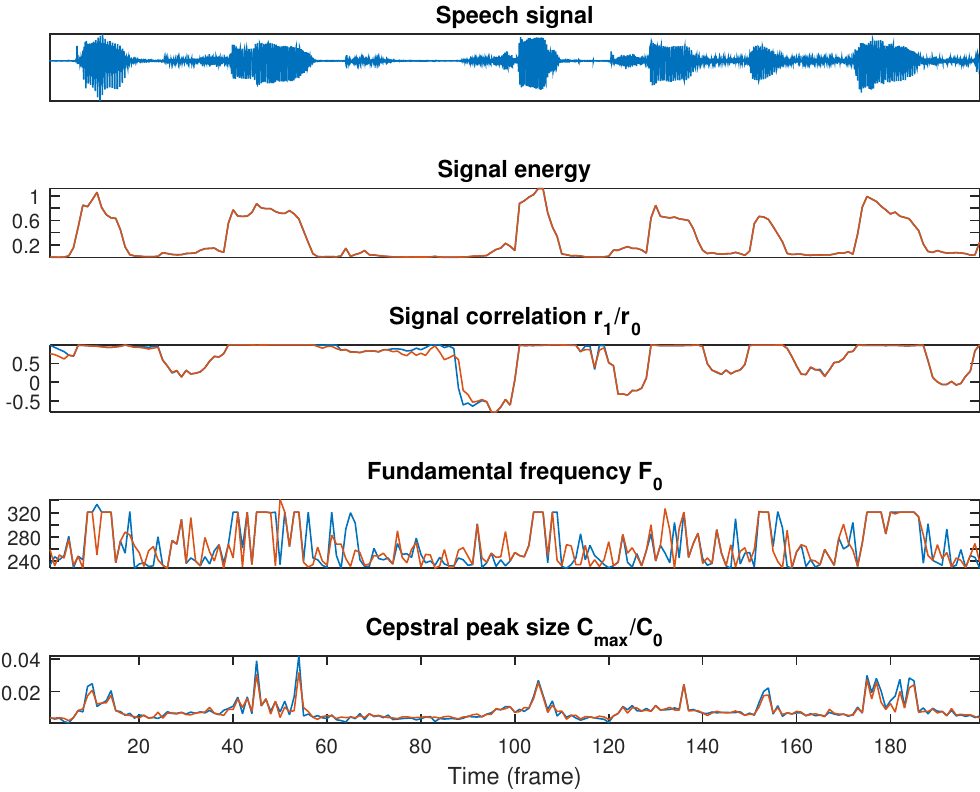
• In VAD, with features we try to measure some property of the signal which would give an indication to whether the signal is speech or non-speech.

  • Signal energy is naturally a useful feature, since the energy of speech varies a lot.

  • Voiced sounds generally have energy mainly at the low frequencies, whereby estimators for spectral tilt are often useful. For example,

    • Zero-crossings (per time unit) is high for high-frequency signals (noise) and low for low-frequency signals (voiced speech), whereby it can be used as a feature.

    • The lag-1 autocorrelation is high (close to one) for low-frequency signals and low (close to -1) for high-frequency signals.

• Speech sounds can be efficiently modelled by linear prediction.

  • If the prediction error is small, then it is likely that the signal is speech.

  • If the prediction error is large, then it is probably non-speech.

• Voiced speech has by definition a prominent pitch.

  • If we can identify a prominent pitch in the range then it is likely voiced speech.

• Speech information is described effectively by their spectral envelope.

  • MFCC can be used as a description of envelope information and it is thus a useful set of features.

  • Linear prediction parameters (esp. prediction residual) also describe envelope information and can thus also be used as a feature-set.

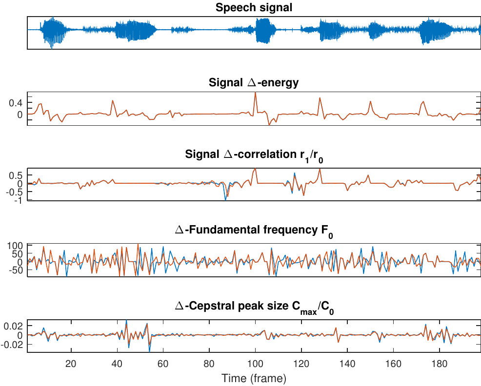
• Speech features vary rapidly and frequently.

  • By looking at the rate of change \(\Delta_k=f_{k+1}-f_k\) in other features \(f_k\), we obtain information about the rate of change of the signal. (Estimate of derivative)

  • Likewise, we can look at the second difference \(\Delta\Delta_k=\Delta_{k+1}-\Delta_k\). (Estimate of second derivative)

  • These first and second order differences can be used as features and they are known as \(\Delta\)- and \(\Delta\Delta\)-features.

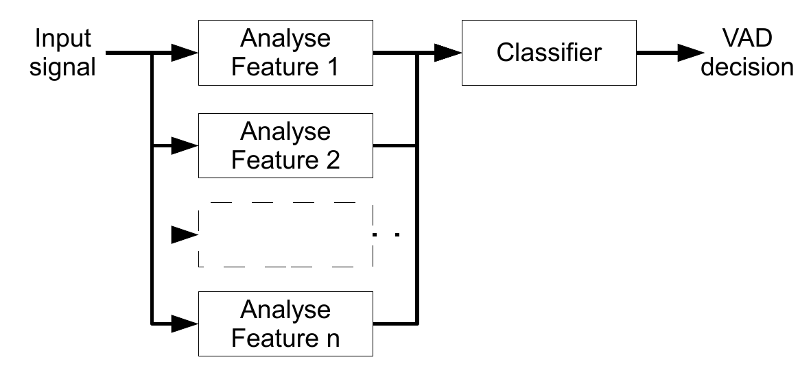
8.1.6. Classifier

• We have collected a set of indicators for speech, the features, whereby the next step is to merge the information from these features to make a decision between speech and non-speech.

• Classification is generic problem, with plenty of solutions such as

  • decision trees (low-complexity, requires manual tuning)

  • linear classifier (relatively low-complexity, training from data)

  • deep neural networks (high-complexity, high-accuracy, training from data)

The following examples use deep neural networks from SpeechBrain.

from speechbrain.inference.VAD import VAD

file1 = "sounds/vad_test1.wav"

VAD = VAD.from_hparams(source="speechbrain/vad-crdnn-libriparty", savedir="pretrained_models/vad-crdnn-libriparty")
boundaries = VAD.get_speech_segments(file1)
VAD.save_boundaries(boundaries)

prob_chunks = VAD.get_speech_prob_file(file1)

/u/14/backstt1/unix/anaconda3/envs/itsp2025/lib/python3.12/site-packages/speechbrain/utils/autocast.py:188: FutureWarning: `torch.cuda.amp.custom_fwd(args...)` is deprecated. Please use `torch.amp.custom_fwd(args..., device_type='cuda')` instead.
  wrapped_fwd = torch.cuda.amp.custom_fwd(fwd, cast_inputs=cast_inputs)

segment_001  0.00  2.70 NON_SPEECH
segment_002  2.70  5.88 SPEECH
segment_003  5.88  7.40 NON_SPEECH
segment_004  7.40  10.55 SPEECH

Show code cell source Hide code cell source

plt.figure(figsize=(12,3))
fs, data = wavfile.read(file1)
data = data[:]
t = np.arange(0,len(data),1)/fs

plt.subplot(211)
plt.plot(t,data,label='Waveform')
plt.ylabel('Amplitude')
plt.title('Speech signal')
plt.axis([0, len(data)/fs, -1.05*np.max(np.abs(data)), 1.05*np.max(np.abs(data))])
plt.legend()


plt.subplot(212)
t = np.linspace(0,1,num=prob_chunks.squeeze().shape[0])*len(data)/fs
plt.plot(t,prob_chunks.squeeze(),label='VAD Output')
plt.ylabel('Amplitude')
plt.axis([0, len(data)/fs, -.1, 1.15])
plt.legend()

plt.tight_layout()
plt.show()

ipd.display(ipd.Audio(data,rate=fs))

file2 = "sounds/vad_test2.wav"

VAD = VAD.from_hparams(source="speechbrain/vad-crdnn-libriparty", savedir="pretrained_models/vad-crdnn-libriparty")
boundaries = VAD.get_speech_segments(file2)
VAD.save_boundaries(boundaries)

prob_chunks = VAD.get_speech_prob_file(file2)

Show code cell source Hide code cell source

plt.figure(figsize=(12,5))
plt.subplot(211)
fs, data = wavfile.read(file2)
data = data[:]
t = np.arange(0,len(data),1)/fs

plt.plot(t,data,label='Waveform')
plt.ylabel('Amplitude')
plt.title('Speech signal')
plt.axis([0, len(data)/fs, -1.05*np.max(np.abs(data)), 1.05*np.max(np.abs(data))])
plt.legend()


plt.subplot(212)
t = np.linspace(0,1,num=prob_chunks.squeeze().shape[0])*len(data)/fs
plt.plot(t,prob_chunks.squeeze(),label='VAD Output')
plt.ylabel('Amplitude')
plt.axis([0, len(data)/fs, -.1, .5])
plt.legend()

plt.tight_layout()
plt.show()


ipd.display(ipd.Audio(data,rate=fs))

The two above examples demonstrate that VAD in noise is a difficult problem.

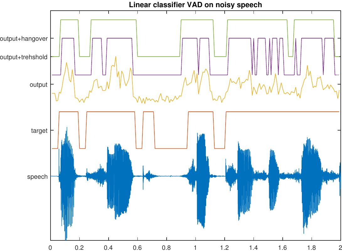
8.1.7. Speech Presence Probability

• The output of the classifier is a continuous number, but it is thresholded to obtain a decision.

• The continuous output contains a lot of information about the signal which is lost when applying thresholding.

  • With a high value we are really certain that the signal is speech, while a value near the threshold is relatively uncertain.

• We can use the classifier output as an estimate of the probability that the signal is speech \(\Rightarrow\) It is an estimator for speech presence probability.

• Subsequent applications can use this information as input to improve performance.

8.1.7.1. Output before thresholding

8.1.8. Noise types

• As noted before, VAD is trivial in noise-free scenarios.

• In practice, typical background noise types are for example, office noise, car noise, cafeteria (babble) noise, street noise, factory noise, …

• Clearly the problem is easier if the noise has a very different character than the speech signal.

  • Speech is quickly varying \(\Rightarrow\) stationary noises are easy.

  • Speech is dominated by low frequencies \(\Rightarrow\) high frequency noises are easy.

• The classic worst case is a competing (undesired) speaker, when someone else is speaking in the background (babble noise).

  • However, that would be difficult also for a human listener, whereby it actually is a very difficult problem.

8.1.9. Conclusions

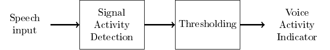
• Voice activity detection is a type of methods which attempt to determine if a signal is speech or non-speech.

  • In a noise-free scenario the task is trivial, but it is also not a realistic scenario.

• The basic idea of algorithms is:

  1. Calculate a set of features from the signal which are designed to analyze properties which differentiate speech and non-speech.

  2. Merge the information from the features in a classifier, which returns the likelihood that the signal is speech.

  3. Threshold the classifier output to determine whether the signal is speech or not.

• VADs are used as a low-complexity pre-processing method, to save resources (e.g. complexity or bitrate) in the main task.

8.1.10. See also

The SpeechBrain project has a nice introduction to VAD.