8.4. Speaker Recognition and Verification#
8.4.1. Introduction to Speaker Recognition#
Speaker recognition is the task of identifying a speaker using their voice. Speaker recognition is classified into two parts: speaker identification and speaker verification. While speaker identification is the process of determining which voice in a group of known voices best matches the speaker’, speaker verification is the task of accepting or rejecting the identity claim of a speaker by analyzing their acoustic samples. Speaker verification systems are computationally less complex than speaker identification systems since they require a comparison between only one or two models, whereas speaker identification requires comparison of one model to N speaker models.
Speaker verification methods are divided into text-dependent and text-independent methods. In text-dependent methods, the speaker verification system has prior knowledge about the text to be spoken and the user is expected to speak this text. However, in a text-independent system, the system has no prior knowledge about the text to be spoken and the user is not expected to be cooperative. Text-dependent systems achieve high speaker verification performance from relatively short utterances, while text-independent systems require long utterances to train reliable models and achieve good performance.
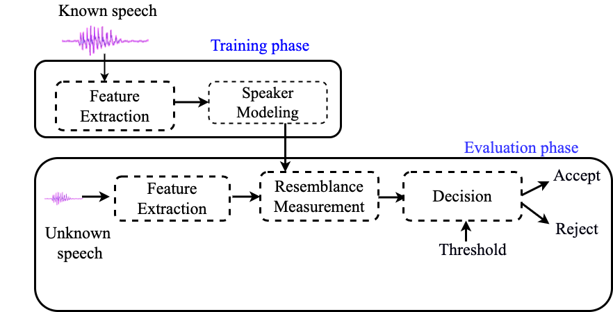 Block diagram of a basic speaker verification system
As it is shown in the above block diagram of a basic speaker verification system, a speaker verification system involves two main phases: the training phase in which the target speakers are enrolled and the testing phase in which a decision about the identity of the speaker is taken. From a training point of view, speaker models can be classified into generative and discriminative. Generative models such as Gaussian Mixture Model (GMM) estimate the feature distribution within each speaker. Discriminative models such as Support Vector Machine and Deep Neural Network (DNN), in contrast, model the boundary between speakers.
The performance of speaker verification systems is degraded by the variability in channels and sessions between enrolment and verification speech signals. Factors which affect channel/session variability include:
Channel mismatch between enrolment and verification speech signals such as using different microphones in enrolment and verification speech signals.
Environmental noise and reverberation conditions.
The differences in speaker voice such as ageing, health, speaking style and emotional state.
Transmission channel such as landline, mobile phone, microphone and voice over Internet protocol (VoIP).
8.4.2. Front-end Processing#
Many front-end processing are often used to process the speech signals and to extract the features which are used in the speaker verification system. The front-end processing consists of mainly voice activity detection (VAD), feature extraction and channel compensation techniques;
Voice activity detection (VAD); The main goal of voice activity detection is to determine which segments of a signal are speech and non-speech. A robust VAD algorithm can improve the performance of a speaker verification system by making sure that speaker identity is calculated only from speech regions. Therefore, it is necessary to review the VAD algorithm to overcome the problems in designing a robust speaker verification system. The three widely used techniques for VAD are the following: energy based, model based and hybrid approaches.
Feature extraction techniques are used to transform the speech signals into acoustic feature vectors. Thus, the extracted acoustic features should carry the essential characteristics of the speech signal which recognizes the identity of the speaker by their voice. The aim of feature extraction is to reduce the dimension of acoustic feature vectors by removing unwanted information and emphasizing the speaker-specific information. The MFCCs are commonly used as the feature extraction technique for the modern speaker verification.
Channel compensation techniques are used to reduce the effect of channel mismatch and environmental noise. Channel compensation can be used in different stages of speaker verification such as feature and model domains. Various channel compensation techniques such as cepstral mean subtraction (CMS) , feature warping, cepstral mean variance normalization (CMVN) and relative spectral (RASTA) processing have been used to reduce the effect of channel mismatch during the feature extraction phase. In the model domain, Joint Factor Analysis (JFA) and i-vectors are used to combat enrolment and verification mismatch.
8.4.3. Speaker Modeling Techniques#
One of the crucial issues in speaker diarization is the techniques employed for speaker modeling. Several modeling techniques have been used in speaker recognition and speaker diarization tasks. The state-of-the-art speaker modeling techniques in speaker diarization are the following:
8.4.3.1. Gaussian Mixture Modeling (GMM) - Universal Background Model (UBM) Approach#
A Gaussian Mixture Model (GMM) is a parametric probability density function represented as a weighted sum of Gaussian component densities. GMMs have been successfully used to model the speech features in different speech processing applications. A Gaussian mixture model is a weighted sum of M component Gaussian densities. Each of the components is a multi-variant Gaussian function. A GMM is represented by mean vectors, covariance matrices and mixture weights.
The covariance matrices of a GMM, \( \Sigma_i \) , can be full rank or constrained to be diagonal. The parameters of a GMM can also be shared, or tied, among the Gaussian components. The number of GMM components and type of covariance matrices are often determined based on the amount of data available for estimating GMM parameters.
In speaker recognition, a speaker can be modeled by a GMM from training data or using Maximum A Posteriori (MAP) adaptation. While the speaker model is built using the training utterances of a specific speaker in the GMM training, the model is also usually adapted from a large number of speakers called Universal Background Model in MAP adaptation.
Given a set of training vectors and a GMM configuration, there are several techniques available for estimating the parameters of a GMM . The most popular and used method is the maximum likelihood (ML) estimation.
The ML estimation finds the model parameters that maximize the likelihood of the GMM given a set of data. Assuming an independence between the training vectors \( X = \{x_i,\dots,x_N\} \) , the GMM likelihood is typically described as:
Since direct maximization is not possible on equation on equation 1, the ML parameters are obtained iteratively using expectation-maximization (EM) algorithm. The EM iteratively estimate new model parameters \(\bar{\lambda} \) based on a given model \(\lambda\) such that \(p(X|\bar{\lambda}) \ge p(X|\lambda) \) .
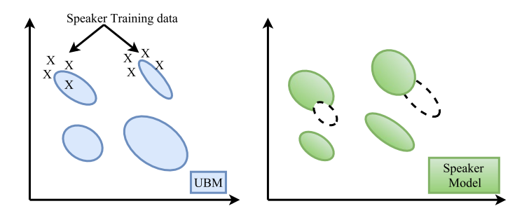 Example of
speaker model adaptation
Example of
speaker model adaptation
The parameters of a GMM can also be estimated using Maximum A Posteriori (MAP) estimation, in addition to the EM algorithm. The MAP estimation technique derives a speaker model by adapting from a universal background model (UBM). The “Expectation” step of EM and MAP are the same. MAP adapts the new sufficient statistics by combining them with old statistics from the prior mixture parameters.
Given a prior model and training vectors from the desired class, \( X = {x_1 . . . , x_T } \) , we first determine the probabilistic alignment of the training vectors into the prior mixture components. For mixture \( i \) in the prior model \( Pr(i|x_t,\lambda_{UBM}) \) is computed as the percentage of the mixture component \( i \) to the total likelihood,
Then, the sufficient statistics for the weight, mean and variance parameters is computed as follows:
Finally, the new sufficient statistics from the training data are used to update the prior sufficient statistics for mixture \( i \) to create the adapted mixture weight, mean and variance for mixture \(i\) as follows:
The adaptation coefficients controlling the balance between old and new estimates are \( \{\alpha^w_i, \alpha^m_i, \alpha^v_i\} \) for the weights, means and variances, respectively. The scale factor, \( \gamma \) , is computed over all adapted mixture weights to ensure they sum to unity.
8.4.3.2. i-Vectors#
Different approaches have been developed recently to improve the performance of speaker recognition systems. The most popular ones were based on GMM-UBM. The Joint Factor Analysis (JFA) is then built on the success of the GMM-UBM approach. JFA modeling defines two distinct spaces: the speaker space defined by the eigenvoice matrix and the channel space represented by the eigen-channel matrix. The channel factors estimated using JFA, which are supposed to model only channel effects, also contain information about speakers. A new speaker verification system has been proposed using factor analysis as a feature extractor that defines only a single space, instead of two separate spaces. In this new space, a given speech recording is represented by a new vector, called total factors as it contains the speaker and channel variabilities simultaneously. Speaker recognition based on the i-vector framework is currently the state-of-the-art in the field.
Given an utterance, the speaker and channel dependent GMM supervector is defined as follows:
where \( m \) is a speaker and channel independent supervector, \( T \) is a rectangular matrix of low rank and \( w \) is a random vector having a standard normal distribution \( N(0,1) \) . The components of the vector \( w \) are the total factors. These new vectors are called i-vectors. \( M \) is assumed to be normally distributed with mean vector and covariance matrix \( TT^t \) .
The total factor is a hidden variable, which can be defined by its posterior distribution conditioned to the Baum–Welch statistics for a given utterance. This posterior distribution is a Gaussian distribution and the mean of this distribution corresponds exactly to i-vector. The Baum–Welch statistics are extracted using the UBM.
Given a sequence of L frames \( \{y_1,y_2,......,y_n\} \) and a UBM \( \Omega \) composed of \( C \) mixture components defined in some feature space of dimension \( F \) , the Baum–Welch statistics needed to estimate the i-vector mixturefor a given speech utterance \( u \) is given by :
where \( m_c \) is the mean of UBM mixture component \( c \) . The i-vector for a given utterance can be obtained using the following equation:
where \( N_u \) is a diagonal matrix of dimension \( CF \times CF \) whose diagonal blocks are \( N_cI(c=1,......, C) \) . The supervector obtained by concatenating all first-order Baum–Welch statistics \( F_c \) for a given utterance \( u \) is represented by \( \hat{F}(u) \) which has \( CF \times 1 \) dimension. The diagonal covariance matrix, \( \Sigma \) , with dimension \( CF \times CF \) estimated during factor analysis training models the residual variability not captured by the total variability matrix \( T \) .
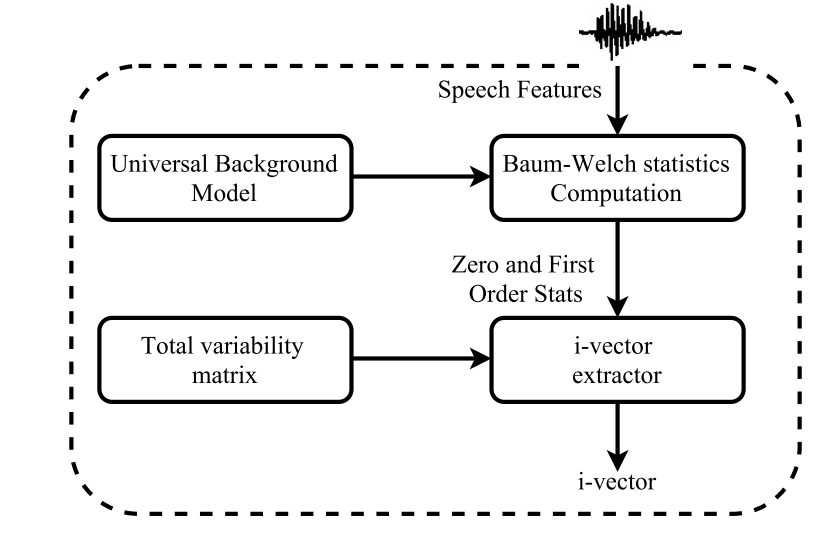 Process of
i-Vector extraction
Process of
i-Vector extraction
One of the most widely used feature normalization techniques of i-vectors is length normalization. Length normalization ensures that the distribution of i-vectors matches the Gaussian normal distribution and makes the distributions of i-vector more similar. Performing whitening before length normalization improves the performance of speaker verification systems. i-vector normalization improves the gaussianity of the i-vectors and reduces the gap between the underlying assumptions of the data and real distributions. It also reduces the dataset shift between development and test i-vectors.
where \( \mu \) and \( \Sigma \) are the mean and the covariance matrix of a training corpus, respectively. The data is standardized according to covariance matrix \( \Sigma \) and length-normalized (i.e., the i-vectors are confined to the hypersphere of unit radius.
The two most widely and common intersession compensation techniques of i-vectors are Within-Class Covariance Normalization (WCCN) and Linear Discriminant Analysis (LDA). WCCN uses the within-class covariance matrix to normalize the cosine kernel functions in order to compensate for intersession variability. LDA attempts to define a reduced special axes that minimize the within-speaker variability caused by channel effects, and maximize between-speaker variability.
8.4.3.2.1. Cosine Distance#
Once the i-vectors are extracted from the outputs of speech clusters, cosine distance scoring tests the hypothesis if two i-vectors belong to the same speaker or different speakers. Given two i-vectors, the cosine distance among them is calculated as follows:
where \( \theta \) is the threshold value, and \( cos(w_i,w_j) \) is the cosine distance score between clusters \( i \) and \( j \) . The corresponding i-vectors extracted for clusters \( i \) and \( j \) are represented by \( w_i \) and \( w_j \) , respectively.
The cosine distance scoring considers only the angle between two i-vectors, not their magnitude. Since the non-speaker information such as session and channel variabilities affect the i-vector magnitude, removing the magnitudes can increase the robustness of i-vector systems.
8.4.3.3. Probabilistic Linear Discriminant Analysis#
The i-vector representation followed by probabilistic linear discriminant analysis (PLDA) modeling technique is the state-of-the-art in speaker verification systems. PLDA has been successfully applied in speaker recognition experiments. It is also applied to handle speaker and session variability in speaker verification task. It has also been successfully applied in speaker clustering since it can separate speaker and noise specific parts of an audio signal which is essential for speaker diarization.
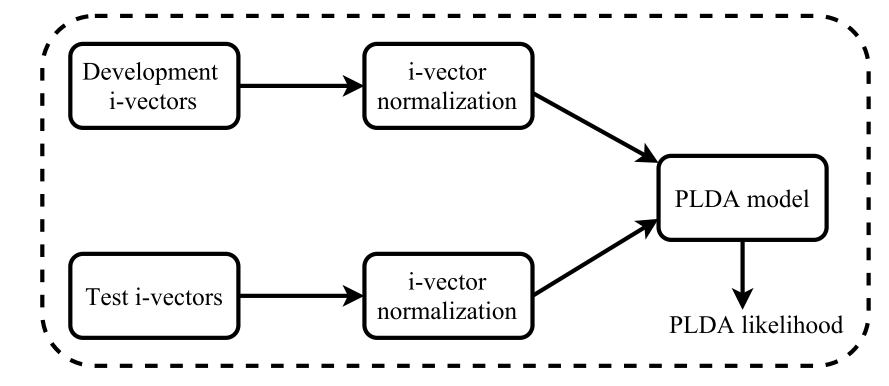 Example of PLDA model
In PLDA, assuming that the training data consists of \(J\) i-vectors where each of these i-vectors belong to speaker \(I\), the \(j\)’th i-vector of the \(I\)th speaker is denoted by:
where \( \mu \) is the overall speaker and segment independent mean of the i-vectors in the training dataset, columns of the matrix F define the between-speaker variability and columns of the matrix G define the basis for the within-speaker variability subspace. \( \Sigma_{ij} \) represents any unexplained data variation. The components of the vector \( h_i \) are the eigenvoice factor loadings and components of the vector \( y_{ij} \) are the eigen-channel factor loadings. The term \( Fh_i \) depends only on the identity of the speaker, not on the particular segment.
Although the PLDA model assumes Gaussian behavior, there is empirical evidence that channel and speaker effects result in i-vectors that are non-Gaussian. It is reported in that the use of Student’s t-distribution, on the assumed Gaussian PLDA model, improves the performance. Since this normalization technique is complicated, a non-linear transformation of i-vectors called radial Gaussianization has been proposed. It whitens the i-vectors and performs length normalization. This restores the Gaussian assumptions of the PLDA model.
A variant of PLDA model called Gaussian PLDA (GPLDA) is shown to provide better results. Because of its low computational requirements, and its performance, it is the most widely used PLDA modeling. In GPLDA model, the within-speaker variability is modeled by a full covariance residual term which allows us to omit the channel subspace. The generative PLDA model for the i-vector is represented by
The residual term \( \Sigma \) representing the within-speaker variability is assumed to have a normal distribution with full covariance matrix \( \Sigma \) .
Given two i-vectors \( w_1 \) and \( w_1 \) , the PLDA computes the likelihood ratio of the two i-vectors as follows:
where the hypothesis \( H_1 \) indicates that both i-vectors belong to the same speaker and \( H_0 \) indicates they belong to two different speakers.
8.4.3.4. Deep Learning (DL)#
The recent advances in computing hardware, new DL architectures and training methods, and access to large amount of training data has inspired the research community to make use of DL technology again as in speaker recognition systems. DL techniques can be used in the frontend or/and backend of a speaker recognition system. The whole end-to-end recognition process can even be performed by a DL architecture.
Deep Learning Frontends: The traditional i-vector approach consists of mainly three stages: Baum-Welch statistics collection, i-vector extraction, and PLDA backend. Recently, it is shown that if the Baum-Welch statistics are computed with respect to a DNN rather than a GMM or if bottleneck features are used in addition to conventional spectral features, a substantial improvement can be achieved. Another possible use of DL in the frontend is to represent the speaker characteristics of a speech signal with a single low dimensional vector using a DL architecture, rather than the traditional i-vector algorithm. These vectors are often referred to as speaker embeddings. Typically, the inputs of the neural network are a sequence of feature vectors and the outputs are speaker classes.
Deep Learning Backends: One of the most effective backend techniques for i-vectors is PLDA which performs the scoring along with the session variability compensation. Usually, a large number of different speakers with several speech samples each are necessary for PLDA to work efficiently. Access to the speaker labeled data is costly and in some cases almost impossible. Moreover, the amount of the performance gain, in terms of accuracy, for short utterances is not as much as that for long utterances. These facts motivated the research community to look for DL based alternative backends. Several techniques have been proposed. Most of these approaches use the speaker labels of the background data for training, as in PLDA, and mostly with no significant gain compared to PLDA.
Deep Learning End-to-Ends: It is also interesting to train an end-to-end recognition system capable of doing multiple stages of signal processing with a unified DL architecture. The neural network will be responsible for the whole process from the feature extraction to the final similarity scores. However, working directly on the audio signals in the time domain is still computationally too expensive and, therefore, the current end-to-end DL systems take mainly the handcrafted feature vectors, e.g., MFCCs, as inputs. Recently, there have been several attempts to build an end-to-end speaker recognition system using DL though most of them focus on text-dependent speaker recognition.
8.4.4. Applications of Speaker Recognition#
Transaction authentication – Toll fraud prevention, telephone credit card purchases, telephone brokerage (e.g., stock trading)
Access control – Physical facilities, computers and data networks
Monitoring – Remote time and attendance logging, home parole verification, prison telephone usage
Information retrieval – Customer information for call centers, audio indexing (speech skimming device), speaker diarization
Forensics – Voice sample matching
8.4.5. Performance Evaluations#
The performance of the speaker verification is measured in terms of errors. The types of error and evaluation metrics commonly used in speaker verification systems are the following.
8.4.6. Types of errors#
False acceptance: A false acceptance occurs when the speech segments from an imposter speaker are falsely accepted as a target speaker by the system.
False rejection: A false rejection occurs when the target speaker is rejected by the verification systems.
8.4.7. Performance metrics#
The performance metrics of speaker verification systems can be measured using the equal error rate (EER) and minimum decision cost function (mDCF). These measures represent different performance characteristics of system though the accuracy of the measurements is based on the number of trials evaluated in order to robustly compute the relevant statistics. Speaker verification performance can also be represented graphically by using the detection error trade-off (DET) plot. The EER is obtained when the false acceptance rate and false rejection rate have the same value. The performance of the system improves if the value of ERR is lower because the sum of total error of the false acceptance and false rejection at the point of ERR decreases. The decision cost function (DCF) is defined by assigning a cost of each error and taking into account the prior probability of target and impostor trails. The decision cost function is defined as:
where \( C_{miss} \) and \( C_{fa} \) are the cost functions of a missed detection and false alarm, respectively. The prior probabilities of target and impostor trails are given by \( P_{target} \) and \( P_{impostor} \) , respectively. The percentages of the missed target and falsely accepted impostors’ trails are represented by \( P_{miss} \) and \( P_{fa} \) , respectively. The mDCF is used to evaluate speaker verification by selecting the minimum value of DCF estimated by changing the threshold value. The mDCF can be used to evaluate speaker verification by selecting the minimum value of DCF estimated by changing the threshold value.
where \( P_{miss} \) and \( P_{fa} \) are the miss and false alarm rates recorded from the trials, and the other parameters are adjusted to suit the evaluation of application-specific requirements.