![]()
3.1. Waveform#
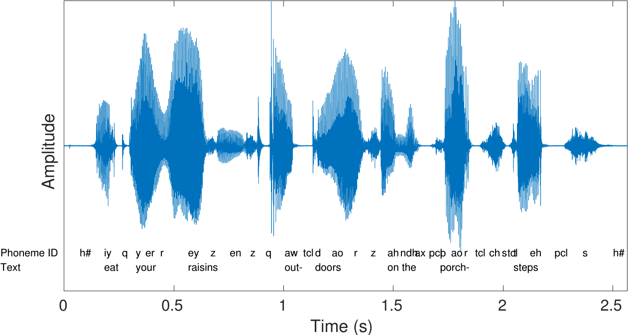
Speech signals are sound signals, defined as pressure variations travelling through the air. These variations in pressure can be described as waves and correspondingly they are often called sound waves. In the current context, we are primarily interested in analysis and processing of such waveforms in digital systems. We will therefore always assume that the acoustic speech signals have been captured by a microphone and converted to a digital form.
A speech signal is then represented by a sequence of numbers \( x_n \) , which represent the relative air pressure at time-instant \( n\in{\mathbb N} \) . This representation is known as pulse code modulation often abbreviated as PCM. The accuracy of this representation is then specified by two factors; 1) the sampling frequency (the step in time between \(n\) and \(n+1\)) and 2) the accuracy and distribution of amplitudes of \(x_n\).
3.1.1. Sampling rate#
Sampling is a classic topic of signal processing. Here the most important aspect is the Nyquist frequency, which is half the sampling rate \(F_s\) and defines the upper end of the largest bandwidth \( \left[0, \frac{F_s}2\right] \) which can be uniquely represented. In other words, if the sampling frequency would be 8000 Hz, then signals in the frequency range 0 to 4000 Hz can be uniquely described with this sampling frequency. The AD-converter would then have to contain a low-pass filter which removes any content above the Nyquist frequency.
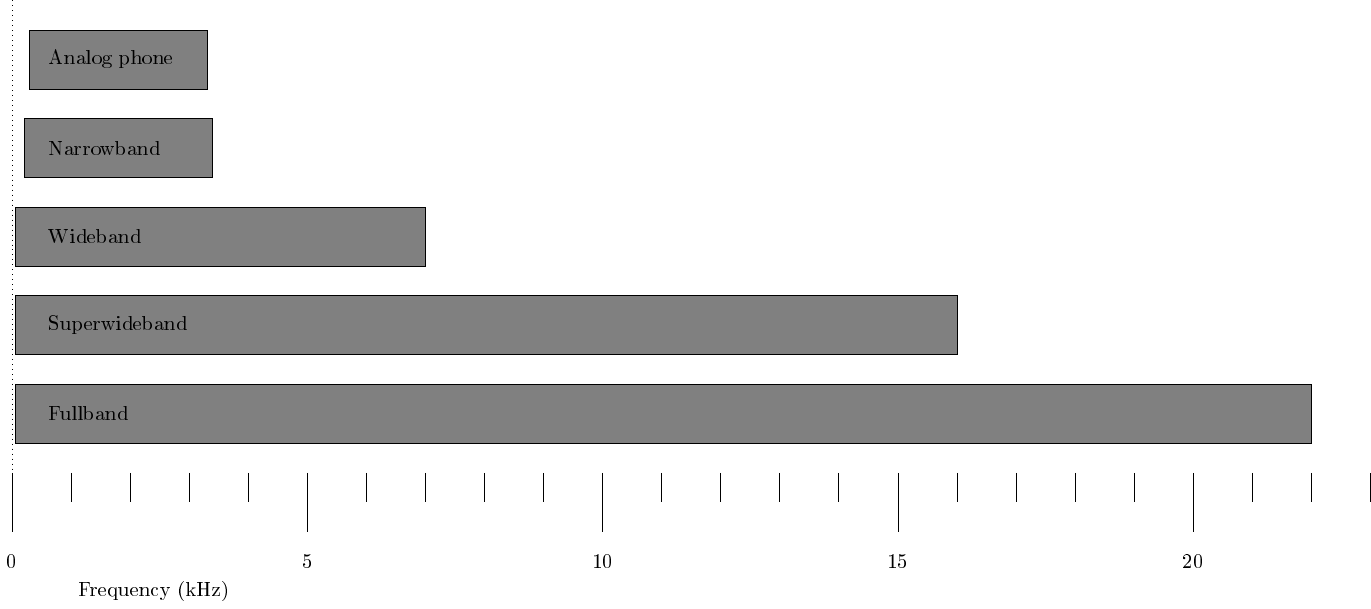
The most important information in speech signals are the formants, which reside in the range 300 Hz to 3500 Hz, such that a lower limit for the sampling rate is around 7 or 8kHz. In fact, first digital speech codecs like the AMR-NB use a sampling rate of 8 kHz known as narrow-band. Some consonants, especially fricatives like /s/, however contain substantial energy above 4kHz, whereby narrow-band is not sufficient for high quality speech. Most energy however remains below 8kHz such that wide-band, that is, a sampling rate of 16 kHz is sufficient for most purposes. Super-wide band and full band further correspond, respectively, to sampling rates of 32 kHz and 44.1 kHz (or 48kHz). The latter is also the sampling rate used in compact discs (CDs). Such higher rates are useful when considering also non-speech signals like music and generic audio.
Frequency-range of different bandwidth-definitions
3.1.2. Static demo#
Sound samples at different bandwidths
Show code cell source
import IPython.display as ipd
import numpy as np
import scipy
from scipy.io import wavfile
from scipy import signal

def bandpass(x,lo,hi):
    X = scipy.fft.dct(x)
    N = len(X)
    X[0:int(lo*N*2)] = 0
    X[int(hi*N*2):] = 0
    return scipy.fft.idct(X)

rate,original = wavfile.read('sounds/speechexample.wav')
ipd.display(ipd.HTML('Original (0 to 22050 Hz)'))
ipd.display(ipd.Audio(original,rate=rate))
ipd.display(ipd.HTML('Narrowband (300 Hz to 3.3 kHz)'))
ipd.display(ipd.Audio(bandpass(original, 300/rate, 3300/rate),rate=rate))
ipd.display(ipd.HTML('Wideband (50 Hz to 7 kHz)'))
ipd.display(ipd.Audio(bandpass(original, 50/rate, 7000/rate),rate=rate))
ipd.display(ipd.HTML('Superwideband (50 Hz to 16 kHz)'))
ipd.display(ipd.Audio(bandpass(original, 50/rate, 16000/rate),rate=rate))
ipd.display(ipd.HTML('Fullband (50 Hz to 22 kHz)'))
ipd.display(ipd.Audio(bandpass(original, 50/rate, 22000/rate),rate=rate))
3.1.3. On-line demo#
Click logo to launch ![]()
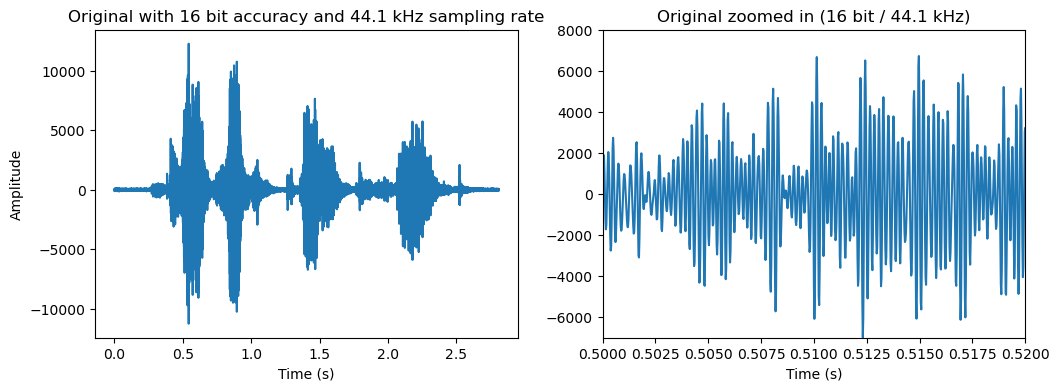
3.1.3.1. Original sound sample#
Show code cell source
from ipywidgets import *
import IPython.display as ipd
import numpy as np
import scipy
from scipy.io import wavfile
from scipy import signal
import matplotlib.pyplot as plt
%matplotlib inline

filename = 'sounds/test.wav'
fs, data = wavfile.read(filename)
data = data.astype(np.int16)

fig = plt.figure(figsize=(12, 4))
ax = fig.subplots(nrows=1,ncols=2)
t = np.arange(0.,len(data))/fs
ax[0].plot(t,data)
ax[0].set_title('Original with 16 bit accuracy and ' + str(fs/1000) + ' kHz sampling rate')
ax[1].plot(t,data)
ax[1].set_title('Original zoomed in (16 bit / ' + str(fs/1000) + ' kHz)')
ax[1].set(xlim=(0.5,0.52),ylim=(-7000,8000))
ax[0].set_xlabel('Time (s)')
ax[1].set_xlabel('Time (s)')
ax[0].set_ylabel('Amplitude')
plt.show()

import IPython.display as ipd
ipd.display(ipd.Audio(filename))
3.1.3.2. Resampling#
Show code cell source
def update(sampling_rate=16000):
    ipd.clear_output(wait=True)
    resample_ratio = sampling_rate/fs
    data_resample = signal.resample(data, int(len(data)*resample_ratio))
    data_resample = signal.resample(data_resample, len(data))
    data_resample = (data_resample*.7*(2**14)/np.max(np.abs(data_resample))).astype(np.int16)
    t = np.arange(0.,len(data_resample))/fs
    fig = plt.figure(figsize=(12, 4))
    ax = fig.subplots(nrows=1,ncols=2)
    ax[0].plot(t,data_resample)
    ax[0].set_title(str(sampling_rate/1000) + ' kHz sampling rate')
    ax[1].plot(t,data_resample)
    ax[1].set_title('Zoom in with ' + str(sampling_rate/1000) + ' kHz')
    ax[1].set(xlim=(0.5,0.52),ylim=(-7000,8000))
    ax[0].set_xlabel('Time (s)')
    ax[1].set_xlabel('Time (s)')
    ax[0].set_ylabel('Amplitude')
    plt.show()
    fig.canvas.draw()
    wavfile.write("sounds/temp.wav", fs, data_resample.astype(np.int16))

    ipd.display(ipd.Audio('sounds/temp.wav'))


interact(update, sampling_rate=(2000, fs, 500));
3.1.4. Accuracy and distribution of steps on the amplitude axis#
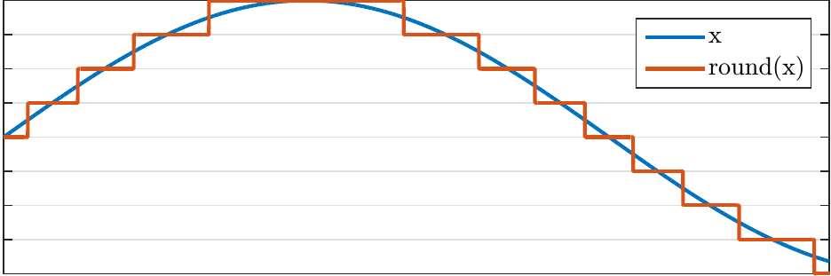
In digital representations of a signal you are forced to use a finite number of steps to describe the amplitude. In practice, we must quantize the signal to some discrete levels.
3.1.4.1. Linear quantization#
Linear quantization with a step size \(\Delta q \) would correspond to defining the quantized signal as
The intermediate representation, \( y={\mathrm{round}}(x/\Delta q),\) can then be taken to represent, for example, signed 16-bit integers. Consequently, the quantization step size \( \Delta q \) has to be then chosen such that \(y\) remains in the range \( y\in(-2^{15},\,2^{15}] \) to avoid numerical overflow.
The beauty of this approach is that it is very simple to implement. The drawback is that this approach is sensitive to the choice of the quantization step size. To make use of the whole range and thus get best accuracy for \(x\), we should choose the smallest \( \Delta q \) where we still remain within the bounds of integers. This is difficult because the amplitudes of speech signals vary on a large range.
Show code cell source
def update(sampling_rate=16000, bits=8):
    ipd.clear_output(wait=True)
    resample_ratio = sampling_rate/fs
    data_resample = signal.resample(data, int(len(data)*resample_ratio))
    data_resample = signal.resample(data_resample, len(data))
    data_resample = (data_resample*.7*(2**14)/np.max(np.abs(data_resample))).astype(np.int16)
    qstep = 2**(16-bits)
    data_q = qstep*np.round(data_resample / qstep)
    t = np.arange(0.,len(data_q))/fs
    fig = plt.figure(figsize=(12, 4))
    ax = fig.subplots(nrows=1,ncols=2)
    ax[0].plot(t,data_q)
    ax[0].set_title(str(bits)+' bit accuracy and ' + str(sampling_rate/1000) + ' kHz sampling rate')
    ax[1].plot(t,data_q)
    ax[1].set_title('Zoom in with '+str(bits)+' bit / ' + str(sampling_rate/1000) + ' kHz')
    ax[1].set(xlim=(0.5,0.52),ylim=(-7000,8000))
    ax[0].set_xlabel('Time (s)')
    ax[1].set_xlabel('Time (s)')
    ax[0].set_ylabel('Amplitude')
    plt.show()
    fig.canvas.draw()
    wavfile.write("temp.wav", fs, data_q.astype(np.int16))

    ipd.display(ipd.Audio('temp.wav'))


interact(update, sampling_rate=(2000, fs, 500), bits=(1,16,1));
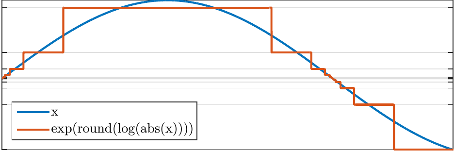
3.1.4.2. Logarithmic quantization and mu-law#
To retain equal accuracy for loud and weak signals, we could quantize on an logarithmic scale as $\( \hat x = {\mathrm{sign}}(x)\cdot\exp\left[ \Delta q\cdot\,{\mathrm{round}} \left(\log\left(\|x\|\right)/\Delta q\right) \right]. \)$ Such operations which limit the detrimental effects of limited range are known as companding algorithms.
Here the intermediate representation is \( y = {\mathrm{round}} \left(\log\left(\|x\|\right)/\Delta q\right) \) which can be reconstructed by \( \hat x = {\mathrm{sign}}(x)\cdot\exp\left[ \Delta q\cdot\,\|y\| \right]. \) A benefit of this approach would be that we can encode signals on a much larger range and the quantization accuracy is relative to the signal magnitude. Unfortunately, very small values cause catastrophic problems. In particular, for \(x=0\), the intermediate value goes to negative infinity \( y=-\infty, \) which is not realizable in finite digital systems.
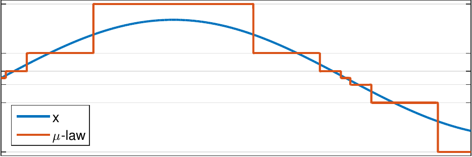
A practical solution to this problem is quantization with the mu-law algorithm, which defines a modified logarithm as
By replacing the logarithm with \(F(x)\), we retain the properties of the logarithm for large \(x\), but avoid the problems when \(x\) is small.
3.1.5. Wav-files#
The most typical format for storing sound signals is the wav-file format. It is basically merely a way to store a time sequence, with typically either 16 or 32 bit accuracy, as integer, mu-law or float. Sampling rates can vary in a large range between 8 and 384 kHz. The files typically have no compression (no lossless nor lossy coding), such that recording hours of sound can require a lot of disk space. For example, an hour of mono (single channel) sound with a sampling rate of 44.1kHz requires 160 MB of disk space.
3.1.6. Adaptive quantization, APCM#
To obtain a uniform quantization error during single phones or sentences, the quantization error has to change slowly over time.
In adaptive quantization (adaptive PCM or APCM) the quantization step size is adapted slowly such that
the available quantization levels cover a sufficient range such that numerical overflow can be avoided,
the quantization error is stable over time and
as long as the above constraints are fulfilled, quantization error is minimized.
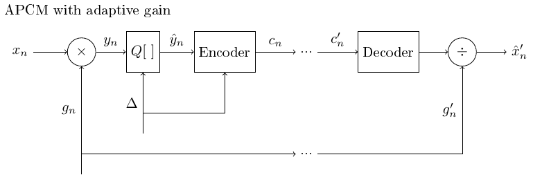
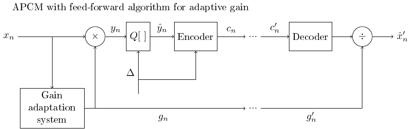
An alternative, equivalent implementation to the change in quantization step size is to apply an adaptive gain to the input signal before quantization.
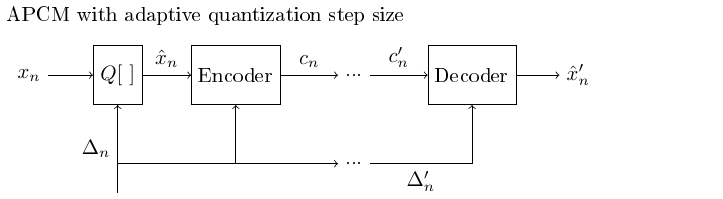
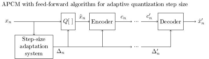
3.1.6.1. Adaptive quantization with the feed-forward algorithm using an adaptive quantization step#
The feed-forward algorithm requires that in addition to the quantized signal, also the gain-coefficients or the quantization step is transmitted to the recipient.
Transmitting such extra information increases the bit-rate, whereby the feed-forward algorithm is not optimal for applications which try to minimize transmission rate.
3.1.6.2. Adaptive quantization with the feed-forward algorithm using an adaptive gain (compressor)#
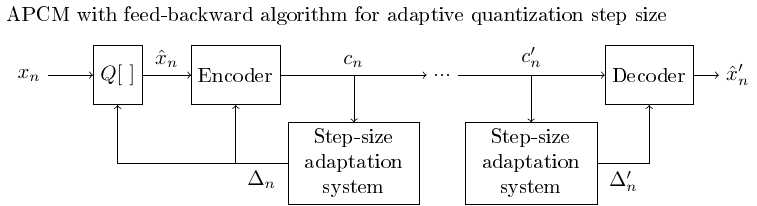
In feed-backward algorithms the quantization step or gain-coefficient is determined from previous samples which are already quantized.
Since the previous samples are available also at the decoder, the quantization step or gain-coefficient can be determined also at the decoder without extra transmitted information.
If the signal grows very rapidly, this approach can however not guarantee that there are no numerical overflows, since adaptation is performed only after quantization.
3.1.6.3. Adaptive quantization with the feed-backward algorithm using an adaptive quantization step#
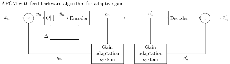
Note that the feed-forward algorithms all require transmission of the scaling or gain coefficient, which can increase demand on bandwidth and adds to the complexity of the system.
The parallel transmission line can be avoided by predicting those coefficients from previously transmitted elements, with a feed-backward algorithm.
3.1.6.4. Adaptive quantization with the feed-backward algorithm using an adaptive gain coefficient#
The feed-backward algorithm can naturally be applied on gain adaptation as well.
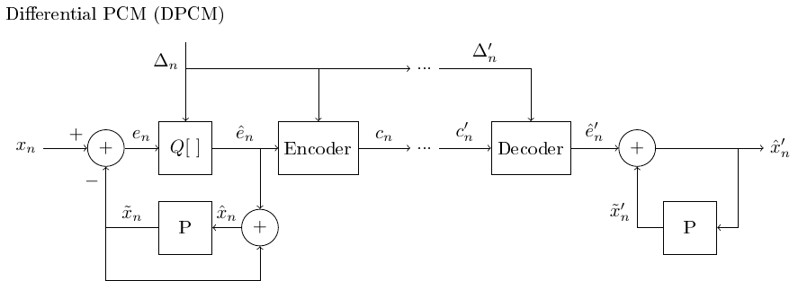
3.1.6.4.1. Differential quantization DPCM#
In differential quantization we predict the subsequent sample, whereby we can quantize only the difference between the prediction and the actual sample.
If the predictor is simply \( \tilde x_k:=x_{k-1}, \) then the error is \( e_k = x_k - \tilde x_k = x_k - x_{k-1}. \)
The first difference (delta modulation) is the simplest predictor, which uses the assumption that subsequent samples are highly correlated.
The reconstruction is obtained by reorganization of terms as \( x_k = e_k + x_{k-1}. \)
Observe that the reconstruction is needed at both the encoder and decoder, to feed the predictor.
NB: At this point the flow-graphs start to get a bit complicated as there are several feedback loops.
More generally, we can use a predictor \(P\), which predicts a sample based on a weighted sum of previous samples
\[ \tilde x_k = -\sum_{h=1}^M a_h x_{k-h}, \]where the scalars \( a_h \) are the predictor parameters.
A feed-backward would here use the past quantized samples \( \hat x_k. \)
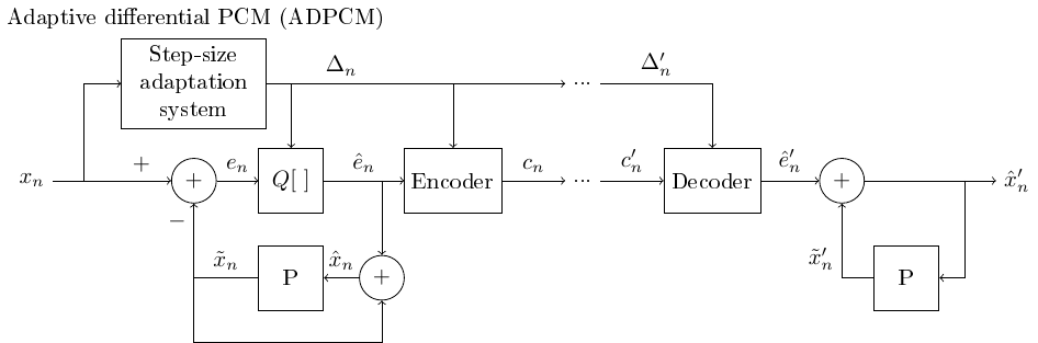
3.1.6.5. Adaptive and differential quantization with feed-forward#
The differential, source-model based quantization can naturally be combined with adaptive, perception-based quantization.
The adaptive differential PCM (ADPCM) adaptively predicts the signal and adaptively choosing the quantization step.
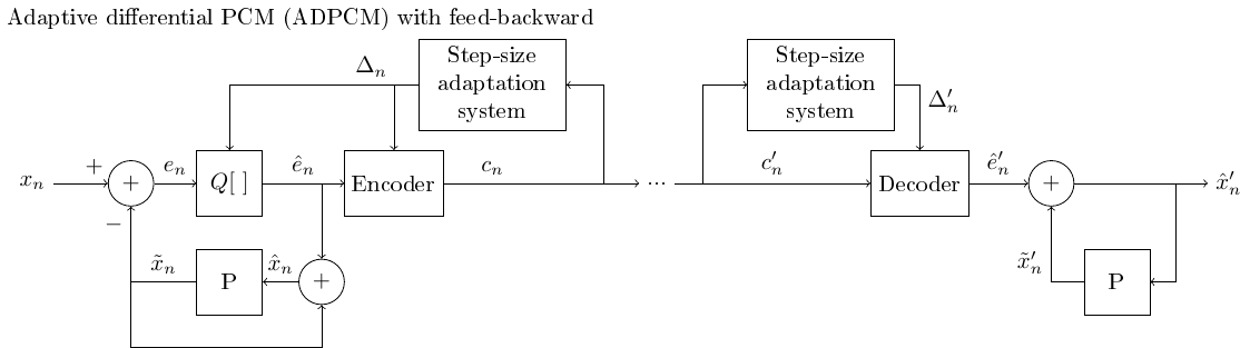
3.1.6.6. Adaptive differential quantization with feed-backward#
The ADPCM can again, naturally, be implemented as a feed-backward algorithm as well.
3.1.6.7. Adaptive differential quantization w/ adaptive predictor#
A differential quantizer can be further improved by letting also the predictor be adaptive.
The predictor learns adaptively properties of the signal.
The flow-graph becomes complicated and is omitted here.
3.1.6.8. Comparison of the SNR of different quantizers (not perceptual)#
The more bits we can use the better the quality (Duh!).
The more prior information we can use about the signal the better the efficiency (SNR/bits).
More advanced models (can) improve quality.
More parameters (can) improve quality.
It would naturally also be entirely possible to create complicated models which do not improve quality, but simple models can go only so far.
The linear prediction -approach can be extended into a full-blown speech production model (see separate chapter).
Note that quality as measured by SNR does not necessarily reflect perceptual quality.
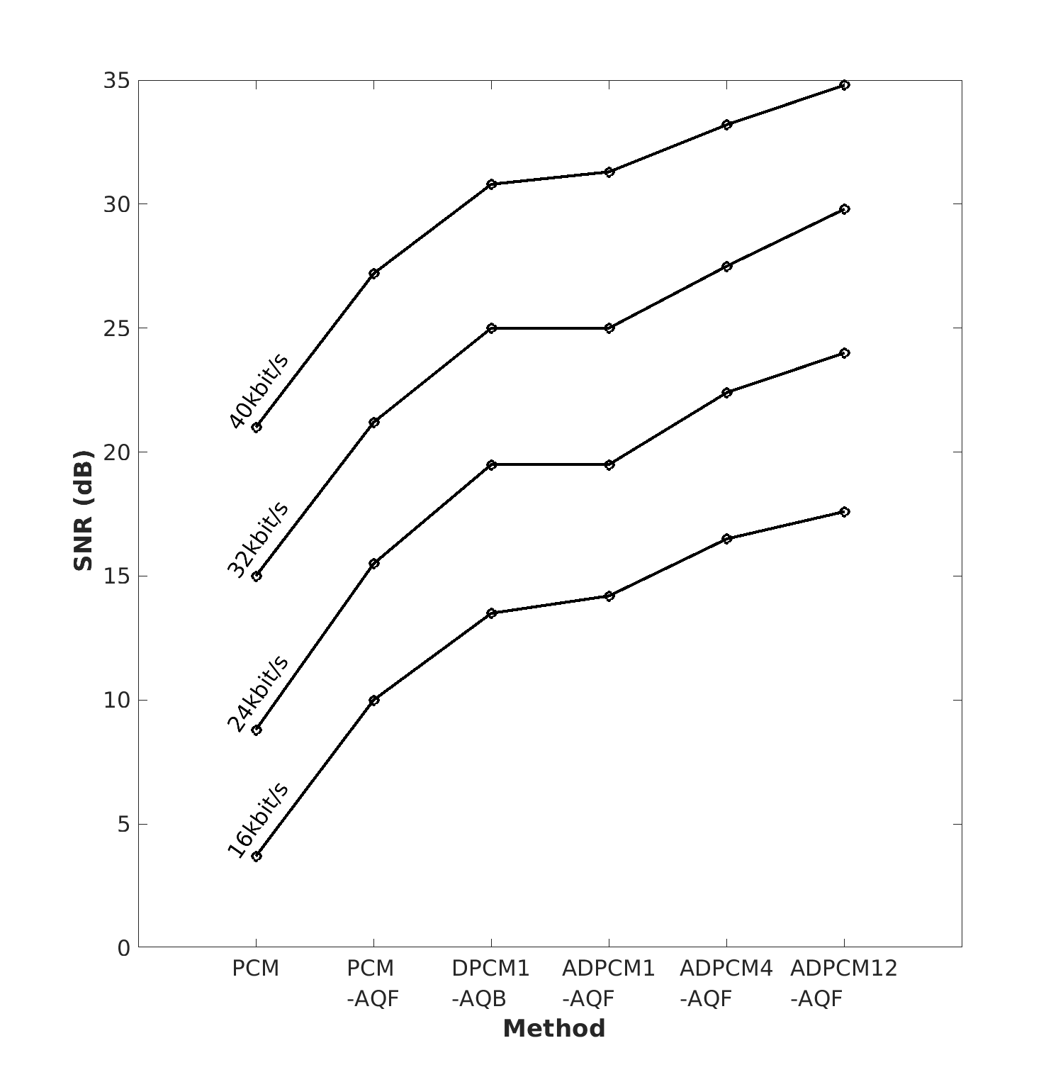 Adapted from [Noll, 1975]
3.1.7. Source modelling in quantization#
Adaptive quantization is based on our understanding of perception; we use the knowledge that we prefer slowly changing quantization errors.
This is a simple perceptual model.
Perceptual models are quality evaluation models.
When we know that the signal is speech, we can use that to further improve quantization.
Models of speech signals are known as source models.
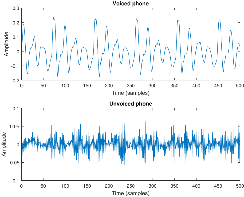
At its simplest form, we can use the fact that voiced phones are fairly continuous signals = they have low-pass character = are dominated by low-frequency components.
Samples have a high correlation.
The difference between subsequent samples is much smaller than the magnitude of samples!
The amplitude of the first difference is 41% of the original.
Uniform quantization of the first difference thus gives a 59% reduction in the range which is approx 1 bitsample. At 44kHz that would be 44kbit/s improvement in bitrate, which is definitely noticeable.
3.1.8. Conclusion#
Time-domain representation of speech signals is simple in floating-point processors.
We only need to choose a sampling rate (typically in the range 8 to 48 kHz).
For fixed-point and lower-bitrate representations, we have several considerations and options;
We would like the quantization noise to be relative to the signal magnitude but stable over time for best perceptual quality.
We can use information about signal properties to improve efficiency with a source model.
If we want to reduce bit-rate, then we must make sure that the required information to decode the signal is available also at the receiving end.
Practical processing algorithms for speech operate on a digital representation of the acoustic signal.
Accuracy is determined by sampling rate and quantization.
Most common (high-quality) storage format for digital speech and audio signals is PCM (such as WAV-files).
Some very basic analysis tools for speech signals include the autocorrelation and the zero-crossing rate.
Many classical DSP algorithms, in their flow-grap representation, are very much alike modern machine learning methods.
3.1.9. Refrences#
Peter Noll. A comparative study of various quantization schemes for speech encoding. Bell System Technical Journal, 54(9):1597 – 1614, 1975. URL: https://doi.org/10.1002/j.1538-7305.1975.tb02053.x.