8.3. Speech Recognition#
8.3.1. Introduction to ASR#
An ASR system produces the most likely word sequence given an incoming speech signal. The statistical approach for speech recognition has dominated Automatic Speech Recognition (ASR) research over the last few decades leading to a number of successes. The problem of speech recognition is defined as the conversion of spoken utterances into textual sentences by a machine. In the statistical framework, the Bayesian decision rule is employed to find the most probable word sequence, \( \hat H \) , given the observation sequence \( O = (o_1, . . . , o_T ) \) :
Following Bayes’ rule, the posterior probability in the above equation can be expressed as a conditional probability of the word sequence given the acoustic observations, \( P(O|H) \) , multiplied by a prior probability of the word sequence, \( P(H) \) , and normalized by the marginal likelihood of observation sequences, \( P(O) \) :
The marginal probability, \( P(O) \) , is discarded in the second equation since it is constant with respect to the ranking of hypotheses, and hence does not alter the search for the best hypothesis. \( P(O|H) \) is calculated by the acoustic model and \( P(H) \) is modeled by the language model.
8.3.2. Component of ASR#
Feature Extraction: It converts the speech signal into a sequence of acoustic feature vectors. These observations should be compact and carry sufficient information for recognition in the later stage.
Acoustic Model: It contains a statistical representation of the distinct sounds that make up each word in the Language Model or Grammar. Each distinct sound corresponds to a phoneme.
Language Model: It contains a very large list of words and their probability of occurrence in a given sequence.
Decoder: It is a software program that takes the sounds spoken by a user and searches the acoustic Model for the equivalent sounds. When a match is made, the decoder determines the phoneme corresponding to the sound. It keeps track of the matching phonemes until it reaches a pause in the users speech. It then searches the language model for the equivalent series of phonemes. If a match is made, it returns the text of the corresponding word or phrase to the calling program.
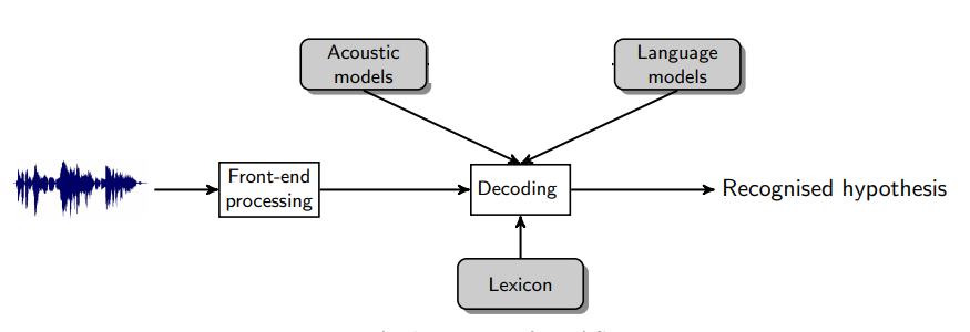 Architecture of an ASR system
8.3.3. Types of ASR#
Speech recognition systems can be classified on the basis of the constraints under which they are developed and which they consequently impose on their users. These constraints include: speaker dependence, type of utterance, size of the vocabulary, linguistic constraints, type of speech and environment of use. We will describe each constraint as follows:
Speaker Dependence: Speaker dependent speech recognition system requires the user to be involved in its development whereas speaker independent systems do not. Speaker independent systems can be used by anybody. Speaker dependent systems usually perform much better than speaker independent systems. This is due to the fact that the acoustic variations among different speakers are very difficult to describe and model. There are approaches to make a system speaker independent. The first one is the use of multiple representations for each reference to capture the speaker variation and the second one is the speaker adaptation approach.
Type of Utterance: A speech recognizer may recognize every word independently. It may require its user to speak each word in a sentence separating them by artificial pause or it may allow the user to speak in a natural way. The first type of system is categorized as an isolated word recognition system. It is the simplest form of a recognition strategy. It can be developed using word-based acoustic models without any language model. If, however, the vocabulary increases sentences composed of isolated words to be recognized, the use of sub-word acoustic models and language models become important. The second one is the continuous speech recognition systems. It allows the users to utter the message in a relatively or completely unconstrained manner. Such recognizers must be capable of performing well in the presence of all the co-articulatory effects. Developing continuous speech recognition systems is, therefore, the most difficult task. This is due to the following properties of continuous speech: word boundaries are unclear in continuous speech; and co-articulatory effects are much stronger in continuous speech
Vocabulary Size: The number of words in the vocabulary is a constraint that makes a speech recognition system small, medium or large. As a rule of thumb, small vocabulary systems are those which have a vocabulary size in the range of 1-99 words; medium, 100-999 words; and large, 1000 words or more. Large vocabulary speech recognition systems perform much worse compared to small vocabulary systems due to different factors such as word confusion that increases with the number of words in the vocabulary. For small vocabulary recognizer, each word can be modeled. However, it is not possible to train acoustic models for thousands of words separately because we cannot have enough training speech and storage for parameters of the speech that is needed. The development of large vocabulary recognizer, therefore, requires the use of sub-word units. On the other hand, the use of sub-word units results in performance degradation since they cannot capture co-articulatory effects as words do. The search process in large vocabulary recognizer also uses pruning instead of performing a complete search.
Type of Speech: A speech recognizer can be developed to recognize only read speech or to allow the user speak spontaneously. The latter is more difficult to build than the former due to the fact that spontaneous speech is characterized by false starts, incomplete sentences, unlimited vocabulary and reduced pronunciation quality. The primary difference in recognition error rates between read and spontaneous speech are due to disfluencies in spontaneous speech. Disfluencies in spontaneous speech can be characterized by long pauses and mispronunciations. Spontaneous is, therefore, both acoustically and grammatically difficult to recognize.
Environment: Speech recognizer may require the speech to be clean from environmental noises, acoustic distortions, microphones and transmission channel distortions or they may ideally handle any of these problems. While current speech recognizer give acceptable performance in carefully controlled environments, their performance degrades rapidly when they are applied in noisy environments. This noise can take the form of speech from other speakers; equipment sounds, air conditioners or others. The noise might also be created by the speaker himself in a form of lip smacks, coughs or sneezes.
8.3.4. Models for Large Vocabulary Speech Recognition (LVCSR)#
LVCSR can be divided into two categories: HMM-based model and the end-to-end model.
8.3.4.1. HMM-Based Model#
The HMM-based model has been the main LVCSR model for many years with the best recognition accuracy. An HMM-based model is divided into three parts:acoustic, pronunciation and language model. In HMM based model, each model is independent of each other and plays a different role. While the acoustic model models the mapping between speech input and feature sequence, the pronunciation model maps between phonemes (or sub-phonemes) to graphemes, and the language model maps the character sequence to fluent final transcription.
Acoustic Model: In the acoustic model, the observation probability is generally represented by GMM. The posterior probability distribution of hidden state can be calculated by DNN method. These two different calculations result into two different models, namely HMM-GMM and HMM-DNN. HMM-GMM model was a general structure for many speech recognition systems. However, with the development of deep learning technology, DNN is introduced into speech recognition for acoustic modeling. DNN has been used to calculate the posterior probability of the HMM state replacing the conventional GMM observation probability. Thus, HMM-GMM model is replaced by HMM-DNN since HMM-GMM provides better results compared to HMM-GMM and becomes state-of-the-art ASR model. In the HMM-based model, different modules use different technologies and have different roles. While the HMM is mainly used to do dynamic time warping at the frame level, GMM and DNN are used to calculate emission probability of HMM hidden states.
Pronunciation Model: Its main objective is achieve the connection between acoustic sequence and language sequence. The dictionary includes various levels of mapping, such as pronunciation to phone, phone to trip-hone. The dictionary is used to achieve structural mapping and map the probability calculation relationship.
Language Model: It contains rudimentary syntactic information. Its aim is to predict the likelihood of specific words occurring one after another in a given language. Typical recognizers use n-gram language models. An n-gram contains the prior probability of the occurrence of a word (unigram), or of a sequence of words (bigram, trigram etc.):
unigram probability \( P(w_i) \)
bigram probability \( P(w_i|w_{i−1}) \)
ngram probability \( P(w_n|w_{n−1},w_{n−2}, …,w_1) \)
Limitations of HMM-models
The training process is complex and difficult to be globally optimized. HMM-based model often uses different training methods and data sets to train different modules. Each module is independently optimized with their own optimization objective functions which are generally different from the true LVCSR performance evaluation criteria. So the optimality of each module does not necessarily bring global optimality.
Conditional independence assumptions. To simplify the model’s construction and training, the HMM-based model uses conditional independence assumptions within HMM and between different modules. This does not match the actual situation of LVCSR.
8.3.4.2. End-to-End Model#
Because of the above-mentioned shortcomings of the HMM-based model and coupled with the promotion of deep learning technology, more and more works began to study end-to-end LVCSR. The end-to-end model is a system that directly maps input audio sequence to sequence of words or other graphemes.
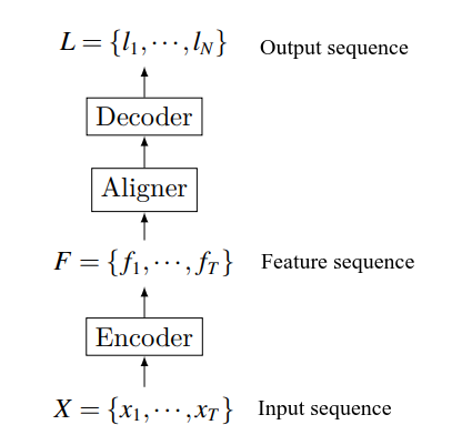 Function structure of end-to-end model
Most end-to-end speech recognition models include the following parts: the encoder maps speech input sequence to feature sequence; the aligner realizes the alignment between feature sequence and language; the decoder decodes the final identification result. Note that this division does not always exist since end-to-end itself is a complete structure. Contrary to the HMM-based model that consists of multiple modules, the end-to-end model replaces multiple modules with a deep network, realizing the direct mapping of acoustic signals into label sequences without carefully-designed intermediate states. In addition to this, there is no need to perform posterior processing on the output.
Compared to HMM-based model, the main characteristics of end-to-end LVCSR are:
Multiple modules are merged into one network for joint training. The benefit of merging multiple modules is there is no need to design many modules to realize the mapping between various intermediate states. Joint training enables the end-to-end model to use a function that is highly relevant to the final evaluation criteria as a global optimization goal, thereby seeking globally optimal results.
It directly maps input acoustic signature sequence to the text result sequence, and does not require further processing to achieve the true transcription or to improve recognition performance . But, in the HMM-based models, there is usually an internal representation for pronunciation of a character chain.
These features of end-to-end LVCSR model enables to greatly simplify the construction and training of speech recognition models.
The end-to-end model are mainly divided into three different categories depending on their implementations of soft alignment:
CTC-based: It first enumerates all possible hard alignments. Then, it achieves soft alignment by aggregating these hard alignments. CTC assumes that output labels are independent of each other when enumerating hard alignments.
RNN-transducer: It also enumerates all possible hard alignments and then aggregates them for soft alignment. But unlike CTC, RNN-transducer does not make independent assumptions about labels when enumerating hard alignments. Thus, it is different from CTC in terms of path definition and probability calculation.
Attention-based: This method no longer enumerates all possible hard alignments, but uses attention mechanism to directly calculate the soft alignment information between input data and output label.
CTC-Based End-to-End Model
Although HMM-DNN provides still state-of-the-art results, the role played by DNN is limited. It is mainly used to model the posterior state probability of HMM’s hidden state. The time-domain feature is still modeled by HMM. When attempting to model time-domain features using RNN or CNN instead of HMM, it faces a data alignment problem: both RNN and CNN’s loss functions are defined at each point in the sequence, so in order to be able to perform training, it is necessary to know the alignment relation between RNN output sequence and target sequence.
CTC makes it possible to make fuller use of DNN in speech recognition and build end-to-end models, which is a breakthrough in the development of end-to-end method. Essentially, CTC is a loss function, but it solves hard alignment problem while calculating the loss. CTC mainly overcomes the following two difficulties for end-to-end LVCSR models:
Data alignment problem. CTC no longer needs to segment and align training data. This solves the alignment problem so that DNN can be used to model time-domain features, which greatly enhances DNN’s role in LVCSR tasks.
Directly output the target transcriptions. Traditional models often output phonemes or other small units, and further processing is required to obtain the final transcriptions. CTC eliminates the need for small units and direct output in final target form, greatly simplifying the construction and training of end-to-end model.
RNN-Transducer End-to-End Model
CTC has two main deficiencies in CTC which hinder its effectiveness:
CTC cannot model interdependencies within the output sequence because it assumes that output elements are independent of each other. Therefore, CTC cannot learn the language model. The speech recognition network trained by CTC should be treated as only an acoustic model.
CTC can only map input sequences to output sequences that are shorter than it. Thus, it is powerless for scenarios where output sequence is longer.
For speech recognition, the first point has huge impact. RNN-transducer was proposed to solve the above-mentioned shortcomings of CTC. Theoretically, it can map an input to any finite, discrete output sequence. Interdependencies between input and output and within output elements are also jointly modeled.
The RNN-transducer has many similarities with CT: their main goals is to solve the forced segmentation alignment problem in speech recognition; they both introduce a “blank” label; they both calculate the probability of all possible paths and aggregate them to get the label sequence. However, their path generation processes and the path probability calculation methods are completely different. This gives rise to the advantages of RNN-transducer over CTC.
8.3.5. Types of errors made by speech recognizers#
Though ASR research has come a long way, today’s systems are far from being perfect. Speech recognizer are brittle and make errors due to various causes. Most errors made by ASR systems fall into one of the following categories:
Out-of-vocabulary (OOV) errors: Current state of the art speech recognizers have closed vocabularies. This means that they are incapable of recognizing words outside their training vocabulary. Besides misrecognition, the presence of an out-of-vocabulary word in input utterance causes the system to err to a similar word in its vocabulary. Special techniques for handling OOV words have been developed for HMM-GMM and neural ASR systems (see, e.g., [Zhang, 2019]).
Homophone substitution: These errors can occur if more than one lexical entry has the same pronunciation (phone sequence), i.e., they are homophones. While decoding, homophones may be confused with one another causing errors. In general, a well-functioning language model should disambiguate homophones based on the context.
Language model bias: Because of an undue bias towards the language model (effected by a high relative weight on the language model), the decoder may be forced to reject the true hypothesis in favor of a spurious candidate with high language model probability. These errors may occur along with analogous acoustic model bias.
Multiple acoustic problems: This is a broad category of errors comprising those due to bad pronunciation entries; disfluency, mispronunciation by the speaker himself/herself, or errors made by acoustic models (possibly due to acoustic noise, data mismatch between training and usage etc.).
8.3.6. Challenges of ASR#
Recent advances in ASR has brought automatic speech recognition accuracy close to human performance in many practical tasks. However, there are still challenges:
Out-of-vocabulary words are difficult to recognize correctly
Varying environmental noises impair recognition accuracy.
Overlapping speech is problematic for ASR system.
Recognizing children’s speech and the speech of people with speech production disabilities is suboptimal with regular training data.
DNN-based models usually require a lot of data for training, in the order of thousands of hours. End-to-end models may need up to 100,000h of speech to reach high performance.
Uncertainty self-awareness is limited: typical ASR systems always output the most likely word sequence instead of reporting if some part of the input was incomprehensible or highly uncertain.
8.3.7. Evaluation#
The performance of an ASR system is measured by comparing the hypothesized transcriptions and reference transcriptions. Word error rate (WER) is the most widely used metric. The two word sequences are first aligned using a dynamic programming-based string alignment algorithm. After the alignment, the number of deletions (D), substitutions (S), and insertions (I) are determined. The deletions, substitutions and insertions are all considered as errors, and the WER is calculated by the rate of the number of errors to the number of words (N) in the reference.
Sentence Error Rate (SER) is also sometime used to evaluate the performance of ASR systems. SER computes the percentage of sentences with at least one error.
8.3.7.1. References#
Xiaohui Zhang. Strategies for Handling Out-of-Vocabulary Words in Automatic Speech Recognition. PhD thesis, Johns Hopkins University, 2019. URL: http://jhir.library.jhu.edu/handle/1774.2/62275.