
11.1. Noise attenuation#
When using speech technology in realistic environments, such as at home, office or in a car, there will invariably be also other sounds present and not only the speech sounds of desired speaker. There will be the background hum of computers and air conditioning, cars honking, other speakers, and so on. Such sounds reduces the quality of the desired signal, making it more strenuous to listen, more difficult to understand or at the worst case, it might render the speech signal unintelligible. A common feature of these sounds is however that they are independent of and uncorrelated with the desired signal. [Benesty et al., 2008]
That is, we can usually assume that such noises are additive, such that the observed signal \(y\) is the sum of the desired signal \(x\) and interfering noises \(v\), that is, \(y=x+v\). To improve the quality of the observed signal, we would like to make an estimate \( \hat x =f(y)\) of the desired signal \(x\). The estimate should approximate the desired signal \( x\approx \hat x \) or conversely, we would like to minimize the distance \( d\left(x,\hat x\right) \) with some distance measure \(d(\cdot,\cdot)\).
The sound sample below serves as an example of a noisy speech signal. In the following sections, we discuss incrementally more advanced approaches for attenuating such additive noise.
# Initialization for all
from scipy.io import wavfile
import numpy as np
import matplotlib.pyplot as plt
import IPython.display as ipd
import scipy
import scipy.fft
#from helper_functions import stft, istft, halfsinewindow
Show code cell source
def stft(data,fs,window_length_ms=30,window_step_ms=20,windowing_function=None):
window_length = int(window_length_ms*fs/2000)*2
window_step = int(window_step_ms*fs/1000)
if windowing_function is None:
windowing_function = np.sin(np.pi*np.arange(0.5,window_length,1)/window_length)**2
total_length = len(data)
window_count = int( (total_length-window_length)/window_step) + 1
spectrum_length = int((window_length)/2)+1
spectrogram = np.zeros((window_count,spectrum_length),dtype=complex)
for k in range(window_count):
starting_position = k*window_step
data_vector = data[starting_position:(starting_position+window_length),]
window_spectrum = scipy.fft.rfft(data_vector*windowing_function,n=window_length)
spectrogram[k,:] = window_spectrum
return spectrogram
def istft(spectrogram,fs,window_length_ms=30,window_step_ms=20,windowing_function=None):
window_length = int(window_length_ms*fs/2000)*2
window_step = int(window_step_ms*fs/1000)
#if windowing_function is None:
# windowing_function = np.ones(window_length)
window_count = spectrogram.shape[0]
total_length = (window_count-1)*window_step + window_length
data = np.zeros(total_length)
for k in range(window_count):
starting_position = k*window_step
ix = np.arange(starting_position,starting_position+window_length)
thiswin = scipy.fft.irfft(spectrogram[k,:],n=window_length)
data[ix] = data[ix] + thiswin*windowing_function
return data
def halfsinewindow(window_length):
return np.sin(np.pi*np.arange(0.5,window_length,1)/window_length)
Show code cell source
fs = 44100 # Sample rate
seconds = 5 # Duration of recording
window_length_ms=30
window_step_ms=15
window_length = int(window_length_ms*fs/2000)*2
window_step_samples = int(window_step_ms*fs/1000)
windowing_function = halfsinewindow(window_length)
filename = 'sounds/enhancement_test.wav'
Show code cell source
# read from storage
fs, data = wavfile.read(filename)
data = data[:]
ipd.display(ipd.Audio(data,rate=fs))
plt.figure(figsize=[12,6])
plt.subplot(211)
t = np.arange(0,len(data),1)/fs
plt.plot(t,data)
plt.xlabel('Time (s)')
plt.ylabel('Amplitude')
plt.title('Waveform of noisy audio')
plt.axis([0, len(data)/fs, 1.05*np.min(data), 1.05*np.max(data)])
spectrogram_matrix = stft(data,
fs,
window_length_ms=window_length_ms,
window_step_ms=window_step_ms,
windowing_function=windowing_function)
fft_length = spectrogram_matrix.shape[1]
window_count = spectrogram_matrix.shape[0]
length_in_s = window_count*window_step_ms/1000
plt.subplot(212)
plt.imshow(20*np.log10(np.abs(spectrogram_matrix[:,range(fft_length)].T)),
origin='lower',aspect='auto',
extent=[0, length_in_s, 0, fs/2000])
plt.axis([0, length_in_s, 0, 8])
plt.xlabel('Time (s)')
plt.ylabel('Frequency (kHz)');
plt.title('Spectrogram of noisy audio')
plt.tight_layout()
plt.show()
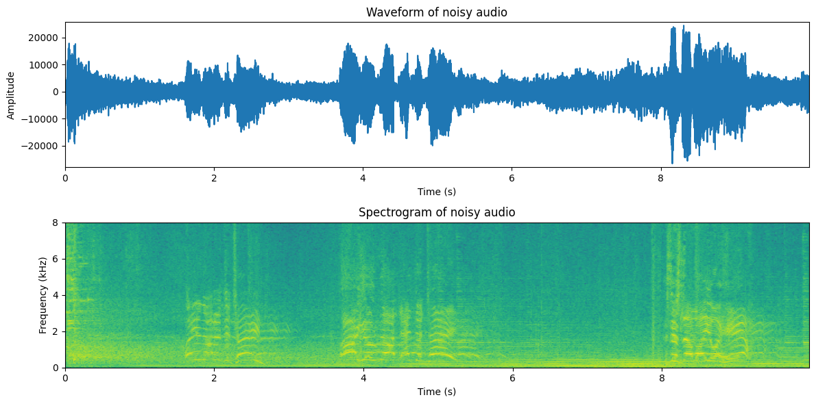
11.1.1. Noise gate#
Suppose you are talking in a reasonably quiet environment. For example, typically when you speak on a phone, you would go to a quiet room. Similarly, when attending an online lecture, you would most often want to be in a room without background noise.
What we perceive as quiet is however never entirely silent. When we play a sound recorded in a “quiet” room, then in the reproduction you then hear the local and the recorded background noises. Assuming the two noises have similar energies, then their sum has twice the energy, viz. 6dB higher than the original noises. In a teleconference with multiple participants, the background noises add up such that each contributes with a 6dB increase in the background noise level. You do not need many participants before the total noise level becomes so high that communication is impossible.
The mute-button in teleconferences is therefore essential. Participants can silence their microphones whenever they are not speaking, such that only the background noise of the active speaker(s) is transmitted to all listeners.
While the mute button is a good user interface in the sense that it gives control to the user, it is however an annoying user interface in that users tend to forget to mute and unmute themselves. Would be better with an automatic mute.
Noise gating is a simple auto-mute in the sense that it thresholds signal energy and turns reproduction/transmission off if energy is too low. Typically it also features a hysteresis functionality such that reproduction/transmission is kept off for a while after the last speech segment. Moreover, to avoid discontinuities, there is a fade-in/fade-out functionality at the start and end.
Note that noise gating with an energy threshold is a simple implementation of a voice activity detector (VAD). With more advanced features than mere energy, we can refine voice activity detection quite a bit, to make it more robust especially in noisy and reverberant environments. In addition to the enhancement of signal quality, such methods are often used also to preserve resources, such as transmission bandwidth (telecommunication) and computation costs (recognition applications such as speech recognition).
For the noise gate, we first need to choose a threshold. Typically the threshold is chosen relative to the mean (log) energy \(\sigma^2\) such that the threshold is \(x^2 < \sigma^2\gamma\), where \(\gamma\) is a tunable parameter. Moreover, we can implement the gate such that if we are below the threshold, we set a gain value to 0 and otherwise to 1. If we want fade-in/fade-out, we can ramp that gain value smoothly from 0 to 1 at the attack and from 1 to 0 at the release.
frame_energy = np.sum(np.abs(spectrogram_matrix)**2,axis=1)
frame_energy_dB = 10*np.log10(frame_energy)
mean_energy_dB = np.mean(frame_energy_dB) # mean of energy in dB
threshold_dB = mean_energy_dB + 3. # threshold relative to mean
speech_active = frame_energy_dB > threshold_dB
Show code cell source
# Reconstruct and play thresholded signal
spectrogram_thresholded = spectrogram_matrix * np.expand_dims(speech_active,axis=1)
data_thresholded = istft(spectrogram_thresholded,fs,window_length_ms=window_length_ms,window_step_ms=window_step_ms,windowing_function=windowing_function)
# Illustrate thresholding (without hysteresis)
plt.figure(figsize=[12,6])
plt.subplot(211)
t = np.arange(0,window_count,1)*window_step_samples/fs
normalized_frame_energy = frame_energy_dB - np.mean(frame_energy_dB)
plt.plot(t,normalized_frame_energy,label='Signal energy')
plt.plot(t,speech_active*10,label='Noise gate')
plt.legend()
plt.xlabel('Time (s)')
plt.ylabel('Amplitude')
plt.title('Noise gate')
plt.axis([0, len(data)/fs, 1.05*np.min(normalized_frame_energy), 1.05*np.max(normalized_frame_energy)])
plt.subplot(212)
plt.imshow(20*np.log10(1e-6+np.abs(spectrogram_thresholded[:,range(fft_length)].T)),
origin='lower',aspect='auto',
extent=[0, length_in_s, 0, fs/2000])
plt.axis([0, length_in_s, 0, 8])
plt.xlabel('Time (s)')
plt.ylabel('Frequency (kHz)');
plt.title('Spectrogram of gated audio')
plt.tight_layout()
plt.show()
#sd.play(data_thresholded,fs)
ipd.display(ipd.Audio(data_thresholded,rate=fs))
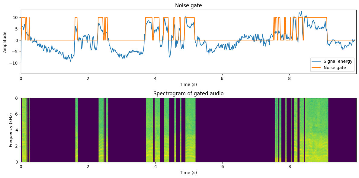
This is quite awful, isn’t it? Though we lost many stationary noise segments, we also distorted the speech signal significantly. In particular, typically we lose plosives at the beginning of words. Overall the sound also sounds odd when it turns on and off again.
To improve, we can add hysteresis, where the activity indicator is kept on for a while after the last true speech frame.
hysteresis_time_ms = 300
hysteresis_time = int(hysteresis_time_ms/window_step_ms)
speech_active_hysteresis = np.zeros([window_count])
for window_ix in range(window_count):
range_start = max(0,window_ix-hysteresis_time)
speech_active_hysteresis[window_ix] = np.max(speech_active[range(range_start,window_ix+1)])
Show code cell source
# Reconstruct and play thresholded signal
spectrogram_hysteresis = spectrogram_matrix * np.expand_dims(speech_active_hysteresis,axis=1)
data_hysteresis = istft(spectrogram_hysteresis,fs,window_length_ms=window_length_ms,window_step_ms=window_step_ms,windowing_function=windowing_function)
# Illustrate thresholding (without hysteresis)
plt.figure(figsize=[12,6])
plt.subplot(211)
t = np.arange(0,window_count,1)*window_step_samples/fs
normalized_frame_energy = frame_energy_dB - np.mean(frame_energy_dB)
plt.plot(t,normalized_frame_energy,label='Signal energy')
plt.plot(t,speech_active_hysteresis*10,label='Noise gate')
plt.legend()
plt.xlabel('Time (s)')
plt.ylabel('Amplitude')
plt.title('Noise gate with hysteresis')
plt.axis([0, len(data)/fs, 1.05*np.min(normalized_frame_energy), 1.05*np.max(normalized_frame_energy)])
plt.subplot(212)
plt.imshow(20*np.log10(1e-6+np.abs(spectrogram_hysteresis[:,range(fft_length)].T)),
origin='lower',aspect='auto',
extent=[0, length_in_s, 0, fs/2000])
plt.axis([0, length_in_s, 0, 8])
plt.xlabel('Time (s)')
plt.ylabel('Frequency (kHz)');
plt.title('Spectrogram of gating with hysteresis')
plt.tight_layout()
plt.show()
#sd.play(data_thresholded,fs)
ipd.display(ipd.Audio(data_hysteresis,rate=fs))
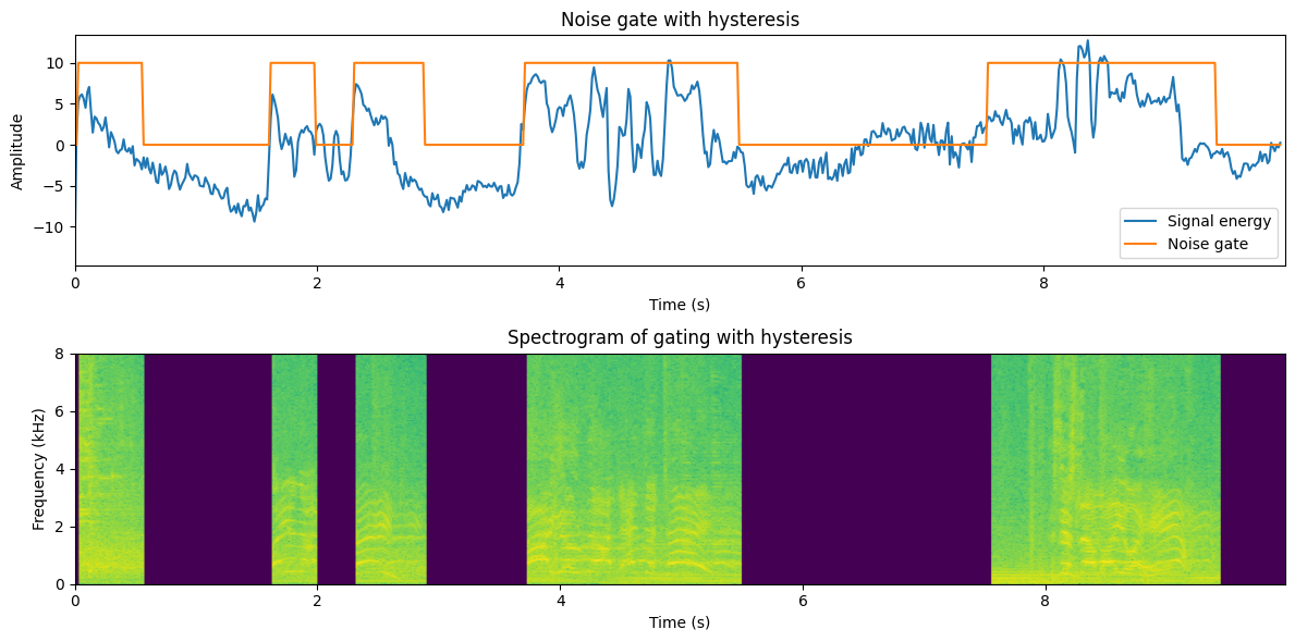
This sounds quite a bit better already. There are only some sudden muted areas (depending on your sound sample), but overall the sound is clearly better.
# Fade-in and fade-out
fade_in_time_ms = 50
fade_out_time_ms = 300
fade_in_time = int(fade_in_time_ms/window_step_ms)
fade_out_time = int(fade_out_time_ms/window_step_ms)
speech_active_sloped = np.zeros([window_count])
for frame_ix in range(window_count):
if speech_active_hysteresis[frame_ix]:
range_start = max(0,frame_ix-fade_in_time)
speech_active_sloped[frame_ix] = np.mean(speech_active_hysteresis[range(range_start,frame_ix+1)])
else:
range_start = max(0,frame_ix-fade_out_time)
speech_active_sloped[frame_ix] = np.mean(speech_active_hysteresis[range(range_start,frame_ix+1)])
Show code cell source
# Reconstruct and play sloped-thresholded signal
spectrogram_sloped = spectrogram_matrix * np.expand_dims(speech_active_sloped,axis=1)
data_sloped = istft(spectrogram_sloped,fs,window_length_ms=window_length_ms,window_step_ms=window_step_ms,windowing_function=windowing_function)
# Illustrate thresholding
plt.figure(figsize=[12,6])
plt.subplot(211)
t = np.arange(0,window_count,1)*window_step_samples/fs
normalized_frame_energy = frame_energy_dB - np.mean(frame_energy_dB)
plt.plot(t,normalized_frame_energy,label='Signal energy')
plt.plot(t,speech_active_sloped*10,label='Noise gate')
plt.legend()
plt.xlabel('Time (s)')
plt.ylabel('Amplitude')
plt.title('Noise gate with sloped hysteresis')
plt.axis([0, len(data)/fs, 1.05*np.min(normalized_frame_energy), 1.05*np.max(normalized_frame_energy)])
plt.subplot(212)
plt.imshow(20*np.log10(1e-6+np.abs(spectrogram_sloped[:,range(fft_length)].T)),
origin='lower',aspect='auto',
extent=[0, length_in_s, 0, fs/2000])
plt.axis([0, length_in_s, 0, 8])
plt.xlabel('Time (s)')
plt.ylabel('Frequency (kHz)');
plt.title('Spectrogram of gating with sloped hysteresis')
plt.tight_layout()
plt.show()
#sd.play(data_thresholded,fs)
ipd.display(ipd.Audio(data_sloped,rate=fs))
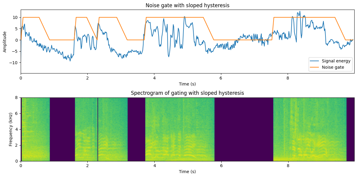
This doesn’t sound all too bad! The sudden on- and off-sets are gone and the transitions to muted areas sound reasonably natural.
Now we have implemented gating for the full-band signal. Gating can be easily improved by band-wise -processing. Depending on the amount of processing you can afford, you could go all the way and apply gating on individual frequency bins in the STFT.
hysteresis_time_ms = 100
hysteresis_time = int(hysteresis_time_ms/window_step_ms)
fade_in_time_ms = 30
fade_out_time_ms = 60
fade_in_time = int(fade_in_time_ms/window_step_ms)
fade_out_time = int(fade_out_time_ms/window_step_ms)
# NB: This is a pedagogic, but very slow implementation since it involves multiple for-loops.
spectrogram_binwise = np.zeros(spectrogram_matrix.shape,dtype=complex)
for bin_ix in range(fft_length):
bin_energy_dB = 10.*np.log10(np.abs(spectrogram_matrix[:,bin_ix])**2)
mean_energy_dB = np.mean(bin_energy_dB) # mean of energy in dB
threshold_dB = mean_energy_dB + 16. # threshold relative to mean
speech_active = bin_energy_dB > threshold_dB
speech_active_hysteresis = np.zeros_like(speech_active)
for window_ix in range(window_count):
range_start = max(0,window_ix-hysteresis_time)
speech_active_hysteresis[window_ix] = np.max(speech_active[range(range_start,window_ix+1)])
#speech_active_sloped = np.zeros_like(spe
for frame_ix in range(window_count):
if speech_active_hysteresis[frame_ix]:
range_start = max(0,frame_ix-fade_in_time)
speech_active_sloped[frame_ix] = np.mean(speech_active_hysteresis[range(range_start,frame_ix+1)])
else:
range_start = max(0,frame_ix-fade_out_time)
speech_active_sloped[frame_ix] = np.mean(speech_active_hysteresis[range(range_start,frame_ix+1)])
spectrogram_binwise[:,bin_ix] = spectrogram_matrix[:,bin_ix]*speech_active_sloped
Show code cell source
# Reconstruct and play sloped-thresholded signal
data_binwise = istft(spectrogram_binwise,fs,window_length_ms=window_length_ms,window_step_ms=window_step_ms,windowing_function=windowing_function)
# Illustrate thresholding
plt.figure(figsize=[12,6])
plt.subplot(211)
plt.imshow(20*np.log10(np.abs(spectrogram_matrix[:,range(fft_length)].T)),
origin='lower',aspect='auto',
extent=[0, length_in_s, 0, fs/2000])
plt.axis([0, length_in_s, 0, 8])
plt.xlabel('Time (s)')
plt.ylabel('Frequency (kHz)');
plt.title('Original spectrogram of noisy audio')
ipd.display(ipd.Audio(data,rate=fs))
plt.subplot(212)
plt.imshow(20*np.log10(1e-6+np.abs(spectrogram_binwise[:,range(fft_length)].T)),
origin='lower',aspect='auto',
extent=[0, length_in_s, 0, fs/2000])
plt.axis([0, length_in_s, 0, 8])
plt.xlabel('Time (s)')
plt.ylabel('Frequency (kHz)');
plt.title('Spectrogram of bin-wise gating with sloped hysteresis')
plt.tight_layout()
plt.show()
#sd.play(data_thresholded,fs)
ipd.display(ipd.Audio(data_binwise,rate=fs))
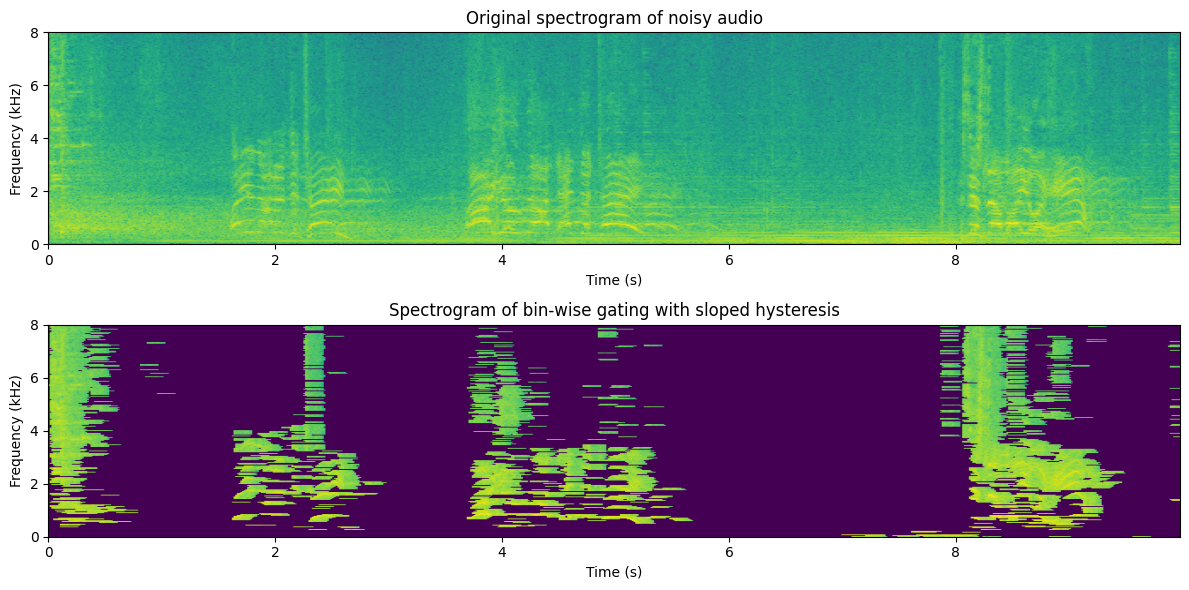
This is clearly again a step better, but you should note two things:
The parameters are now quite a bit different; hysteresis times and ramps are shorter, and the threshold is higher. This was required to get acceptable quality.
Some musical noise is left in the low and high frequencies, where isolated areas are turned on for a while.
If possible, try listening to this sound with headphones and from loudspeakers. Is there a difference? Which one sounds better?
A possible impression is that, with good-quality headphones, the result is too clean. It sounds unnatural. With loudspeakers, however, it may sound quite ok. When listening to headphones, you better perceive the absence of background noise, whereas, on the loudspeaker, there is more background noise present locally, such that the absence of reproduced background noise is not noticeable. With loudspeakers, any reproduced background noise would also interact with the local room, generating a double room reverberation (assuming that the reproduced loudspeaker sound already had reverberation).
In any case, it seems therefore clear that muting the background noise entirely is not always desirable (at least when listening with headphones to a single speaker with background noise). We should therefore apply some more intelligent gain factor (see more in the spectral subtraction section below).
11.1.2. Statistical model#
The STFT spectrum of a signal is a good domain for noise attenuation because we can reasonably safely assume that spectral components are uncorrelated with each other, such that we treat each component separately. In other words, in the spectrum, we can apply noise attenuation on every frequency bin with scalar operations, whereas if the components would be correlated, we would have to use vector and matrix operations. The benefit of scalar operations is that they are computationally simple, \(O(N)\), whereas matrix operations are typically at least \(O(N^2)\).
The sources are, according to our assumption, uncorrelated, which means that the expected correlation is zero,
A consequence of this assumption is that, for the mixture \(y = x + v\), we have the energy expectation
In other words, in terms of expectations, the energy is the sum of component energies, which will become a very useful property.
To find the energy of the speech signal, we then just need to estimate \(E\left[v^2\right]\).
11.1.2.1. Noise estimation and modelling#
11.1.2.1.1. Mean energy with voice activity detection#
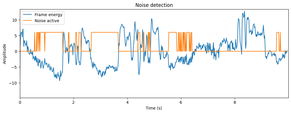
To be able to remove noise, we first need to estimate noise characteristics or statistics. We thus need to find sections of the signal which have noise only (non-speech). One approach would be to use voice activity detection (VAD) to find non-speech segments. Assuming we have a good VAD this can be effective. It works if we assume that noise is stationary, such that the noise on non-speech parts is similar to the noise in speech parts. In general, VADs are accurate only at low noise levels.

# VAD through energy thresholding
frame_energy = np.sum(np.abs(spectrogram_matrix)**2,axis=1)
frame_energy_dB = 10*np.log10(frame_energy)
mean_energy_dB = np.mean(frame_energy_dB) # mean of energy in dB
noise_threshold_dB = mean_energy_dB - 3. # threshold relative to mean
noise_active = frame_energy_dB < noise_threshold_dB
Show code cell source
normalized_frame_energy = frame_energy_dB - mean_energy_dB
plt.figure(figsize=[12,4])
plt.plot(t,normalized_frame_energy,label='Frame energy')
plt.plot(t,noise_active*6,label='Noise active')
plt.legend()
plt.xlabel('Time (s)')
plt.ylabel('Amplitude')
plt.title('Noise detection')
plt.axis([0, len(data)/fs, 1.05*np.min(normalized_frame_energy), 1.05*np.max(normalized_frame_energy)])
plt.show()
# Estimate noise in noise frames
noise_frames = spectrogram_matrix[noise_active,:]
noise_estimate = np.mean(np.abs(noise_frames)**2,axis=0)
Show code cell source
f = np.linspace(0,fs/1000,fft_length)
plt.plot(f,10*np.log10(1e-6+noise_estimate));
plt.xlabel('Frequency (kHz)')
plt.ylabel('Magnitude (dB)');
plt.title('Noise model');
plt.show()
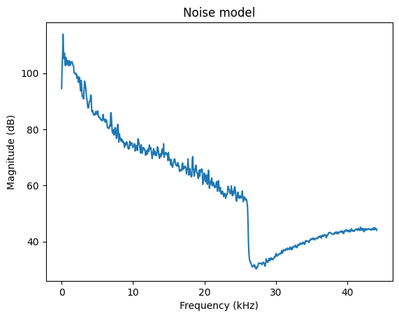
In typical office environments and many other real-world scenarios, the background noise is dominated by low-frequencies, that is, the low frequencies have high energy. Often low-quality hardware also leaks analog distortion into the microphone, such that there can be visible peaks in the higher frequencies.
11.1.2.1.2. Minimum statistics#
An alternative estimate would be the minimum-statistics estimate, where we take the minimum energy of each component over time. Since speech+noise has more energy than just noise alone, the minimum most likely represents only noise. [Martin, 2001]
noise_estimate_minimum = np.min(np.abs(spectrogram_matrix)**2,axis=0)
Show code cell source
plt.plot(f,10*np.log10(noise_estimate),label='Mean+VAD');
plt.plot(f,10*np.log10(noise_estimate_minimum),label='Minimum');
plt.legend()
plt.xlabel('Frequency (kHz)')
plt.ylabel('Magnitude (dB)');
plt.title('Noise models');
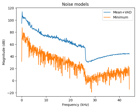
We see that the minimum statistics estimate of noise is much lower than the mean. Duh, it is by definition lower. However, the shape of both spectra is the same. Thus, the minimum statistics estimate is biased but preserves the shape. The bias is something we can correct by adding a fixed constant. The benefit of minimum statistics is that it does not depend on a threshold. We thus replace the threshold parameter with a bias parameter, which is much less prone to errors.
In the following, we will use the mean as our noise model for simplicity.
11.1.3. Spectral subtraction#
The basic idea of spectral subtraction is that we assume that we have access to an estimate of the noise energy \( E[\|v\|^2] = \sigma_v^2\) , and we subtract that from the energy of the observation, such that we define the energy of our estimate as [Boll, 1979]
Unfortunately, since our estimate of noise energy is not perfect and because we have hiddenly made an inaccurate assumption that \(x\) and \(v\) are uncorrelated, the above formula can give negative values for the energy estimate. Negative energy is not realizable and nobody likes pessimists, so we have to modify the formula to threshold at zero
Since STFT spectra are complex-valued, we then still have to find the complex angle of the signal estimate. If the noise energy is small \( \|v\|^2 \ll \|x\|^2 \) , then the complex angle of \(x\) is approximately equal to the angle of \(y\), \( \angle x \approx \angle y \) , such that our final estimate is (when \( \|y\|^2\geq \sigma_v^2 \) )
energy_enhanced = np.subtract(np.abs(spectrogram_matrix)**2, np.expand_dims(noise_estimate,axis=0))
energy_enhanced *= (energy_enhanced > 0) # threshold at zero
enhancement_gain = np.sqrt(energy_enhanced/(np.abs(spectrogram_matrix)**2))
spectrogram_enhanced = spectrogram_matrix*enhancement_gain;
Show code cell source
# Reconstruct and play sloped-thresholded signal
data_enhanced = istft(spectrogram_enhanced,fs,window_length_ms=window_length_ms,window_step_ms=window_step_ms,windowing_function=windowing_function)
# Illustrate thresholding
plt.figure(figsize=[12,6])
plt.subplot(211)
plt.imshow(20*np.log10(np.abs(spectrogram_matrix[:,range(fft_length)].T)),
origin='lower',aspect='auto',
extent=[0, length_in_s, 0, fs/2000])
plt.axis([0, length_in_s, 0, 8])
plt.xlabel('Time (s)')
plt.ylabel('Frequency (kHz)');
plt.title('Original spectrogram of noisy audio')
ipd.display(ipd.Audio(data,rate=fs))
plt.subplot(212)
plt.imshow(20*np.log10(1e-6+np.abs(spectrogram_enhanced[:,range(fft_length)].T)),
origin='lower',aspect='auto',
extent=[0, length_in_s, 0, fs/2000])
plt.axis([0, length_in_s, 0, 8])
plt.xlabel('Time (s)')
plt.ylabel('Frequency (kHz)');
plt.title('Spectrogram after spectral subtraction')
plt.tight_layout()
plt.show()
#sd.play(data_thresholded,fs)
ipd.display(ipd.Audio(data_enhanced,rate=fs))

Typically spectral subtraction does improve the quality of the signal, but it also leaves room for improvement. In particular, usually, we hear musical noise in the higher frequencies, which are components that alternate between on and off. Because these components appear and disappear independently from the speech signal, they are perceived as independent sounds and because they are essentially isolated sinusoids, they are perceived as tones; thus we hear musical, noisy “tones”.
11.1.4. Minimum-mean Square Estimate (MMSE) aka. Wiener filtering#
Observe that the form of the relationship above is \( \hat x = y\cdot g, \) where \(g\) is a scalar scaling coefficient. Instead of the above heuristic, we could then derive a formula that gives the smallest error, for example in the minimum error energy expectation sense or minimum mean square error (MMSE). Specifically, the error energy expectation is
If we assume that target speech and noise are uncorrelated, \( E\left[xv\right]=0 \) ,
then \( E\left[xy\right]=E\left[x(x+v)\right]=E\left[\|x\|^2\right] \) and
The minimum is found by setting the derivative to zero
such that the final solution is
and the Wiener estimate becomes
Observe that this estimate is almost equal to the above, but the square root is omitted. With different optimization criteria, we can easily derive further such estimates. Such estimates have different weaknesses and strengths and it is then a matter of application-specific tuning to choose the best estimate.
Overall, it is however somewhat unsatisfactory that additive noise is attenuated with a multiplicative method. However, without a better model of source and noise characteristics, this is probably the best we can do. Still, spectral subtraction is a powerful method when taking into account how simple it is. With minimal assumptions, we obtain a signal estimate which can give a clear improvement in quality.
mmse_gain = energy_enhanced/(np.abs(spectrogram_matrix)**2)
spectrogram_enhanced_mmse = spectrogram_matrix*mmse_gain
Show code cell source
# Reconstruct and play enhanced signal
data_enhanced_mmse = istft(spectrogram_enhanced_mmse,fs,window_length_ms=window_length_ms,window_step_ms=window_step_ms,windowing_function=windowing_function)
# Illustrate thresholding
plt.figure(figsize=[12,6])
plt.subplot(211)
plt.imshow(20*np.log10(np.abs(spectrogram_matrix[:,range(fft_length)].T)),
origin='lower',aspect='auto',
extent=[0, length_in_s, 0, fs/2000])
plt.axis([0, length_in_s, 0, 8])
plt.xlabel('Time (s)')
plt.ylabel('Frequency (kHz)');
plt.title('Original spectrogram of noisy audio')
ipd.display(ipd.Audio(data,rate=fs))
plt.subplot(212)
plt.imshow(20*np.log10(1e-6+np.abs(spectrogram_enhanced_mmse[:,range(fft_length)].T)),
origin='lower',aspect='auto',
extent=[0, length_in_s, 0, fs/2000])
plt.axis([0, length_in_s, 0, 8])
plt.xlabel('Time (s)')
plt.ylabel('Frequency (kHz)');
plt.title('Spectrogram after Wiener filtering')
plt.tight_layout()
plt.show()
#sd.play(data_thresholded,fs)
ipd.display(ipd.Audio(data_enhanced_mmse,rate=fs))
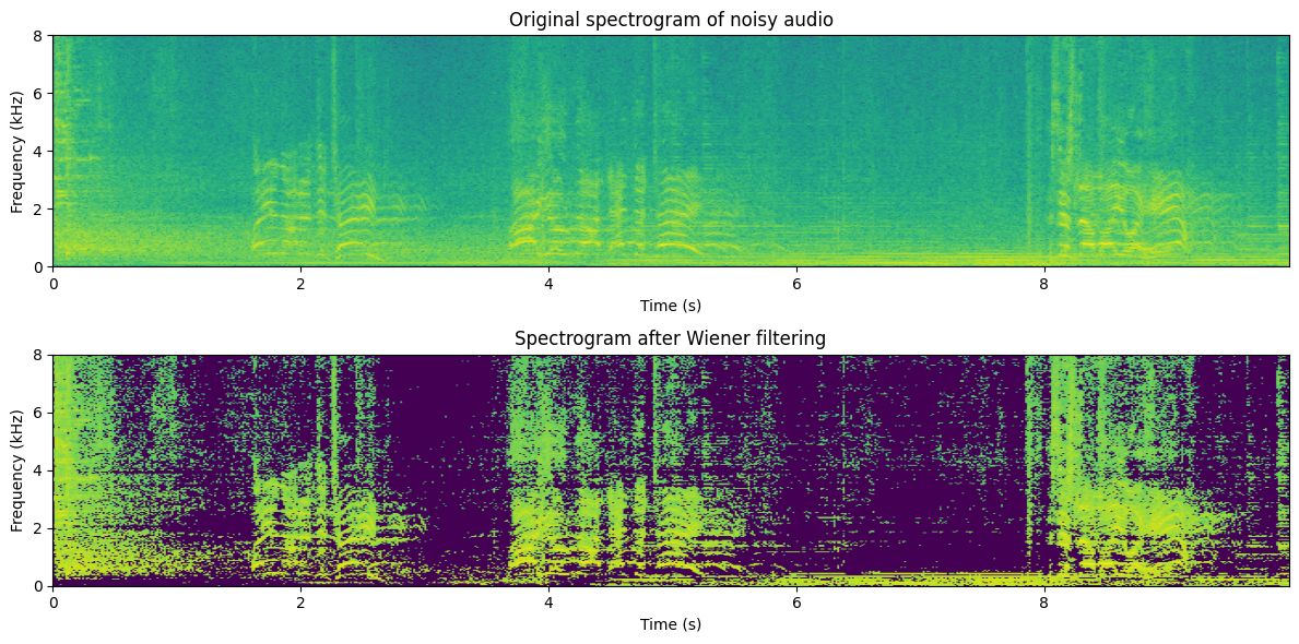
The quality of the MMSE estimate is not drastically different from the spectral subtraction algorithm. This is not surprising as the algorithms are very similar.
In comparison to noise gating, we also notice that it may not be entirely clear which one is better. To a large extent, this will happen with good-quality signals, where the SNR is high. With worse SNR, energy thresholding becomes more difficult and noise gating will surely fail. MMSE is more robust and therefore typically has better quality at low SNR. These methods can also be combined to give the best of both worlds.
11.1.4.1. Treating musical noise#
For spectral-subtraction type methods (which include MMSE), we often encounter musical noise (described above). Similar problems are common in coding applications that use frequency-domain quantization. The problem is related to discontinuity in spectral components over time. Musical noise is perceived when spectral components are randomly turned on and off.
The solution to musical noise must thus be to avoid components going on and off. Possible approaches include:
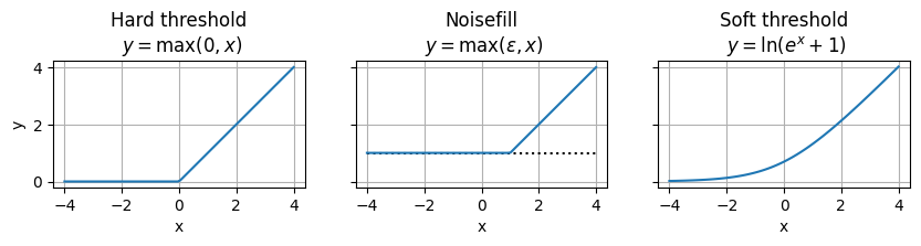
11.1.4.1.1. Noise filling#
Spectral holes (zeros) can be avoided by a noise floor, where we add random noise any time spectral components are below a threshold.
11.1.4.1.2. Mapping#
In spectral-subtraction type methods, the gain value was thresholded at zero before multiplication by the spectrum. It is this thresholding that causes the problem. Therefore, we could replace the hard threshold with a soft threshold. One such soft threshold is the soft-plus, defined for an input \(x\) as \(y=\ln\left(e^x+1\right)\).
Show code cell source
# Illustration of hard threshold, noise filling and soft threshold
noisefill_level = 1
x = np.linspace(-4,4,100)
f, (ax1, ax2, ax3) = plt.subplots(1, 3, sharey=True, figsize=[10,10])
ax1.plot(x,0.5*(x+np.abs(x)))
ax2.plot(x,x*0 + noisefill_level,'k:')
ax2.plot(x,noisefill_level+0.5*(x-noisefill_level+np.abs(x-noisefill_level)))
ax3.plot(x,np.log(1.+np.exp(x)))
ax1.set_title('Hard threshold\n $y=\\max(0,x)$')
ax2.set_title('Noisefill\n $y=\\max(\\epsilon,x)$')
ax3.set_title('Soft threshold\n $y=\\ln(e^x+1)$');
ax1.set_xlabel('x')
ax2.set_xlabel('x')
ax3.set_xlabel('x');
ax1.set_ylabel('y');
ax1.set_aspect('equal')
ax2.set_aspect('equal')
ax3.set_aspect('equal')
ax1.grid()
ax2.grid()
ax3.grid()
plt.show()
# Noise fill with min(eps,x)
noisefill_threshold_dB = -60 # dBs below average noise
noisefill_level = (10**(noisefill_threshold_dB/10))*noise_estimate
#noisefill_level = 0.2
energy_enhanced = np.abs(spectrogram_matrix)**2 - noise_estimate
#energy_noisefill = noisefill_level + 0.5*(energy_enhanced - noisefill_level + np.abs(energy_enhanced - noisefill_level))
energy_noisefill = noisefill_level + ((energy_enhanced - noisefill_level) > 0) * (energy_enhanced - noisefill_level)
mmse_noisefill_gain = np.sqrt(energy_noisefill)/np.abs(spectrogram_matrix)
spectrogram_enhanced_noisefill = spectrogram_matrix*mmse_noisefill_gain;
Show code cell source
# Reconstruct and play enhanced signal
data_enhanced_noisefill = istft(spectrogram_enhanced_noisefill,fs,window_length_ms=window_length_ms,window_step_ms=window_step_ms,windowing_function=windowing_function)
# Illustrate thresholding
plt.figure(figsize=[12,6])
plt.subplot(211)
plt.imshow(20*np.log10(np.abs(spectrogram_matrix[:,range(fft_length)].T)),
origin='lower',aspect='auto',
extent=[0, length_in_s, 0, fs/2000])
plt.axis([0, length_in_s, 0, 8])
plt.xlabel('Time (s)')
plt.ylabel('Frequency (kHz)');
plt.title('Original spectrogram of noisy audio')
ipd.display(ipd.Audio(data,rate=fs))
plt.subplot(212)
plt.imshow(20*np.log10(1e-6+np.abs(spectrogram_enhanced_noisefill[:,range(fft_length)].T)),
origin='lower',aspect='auto',
extent=[0, length_in_s, 0, fs/2000])
plt.axis([0, length_in_s, 0, 8])
plt.xlabel('Time (s)')
plt.ylabel('Frequency (kHz)');
plt.title('Spectrogram after Wiener filtering')
plt.tight_layout()
plt.show()
#sd.play(data_thresholded,fs)
ipd.display(ipd.Audio(data_enhanced_noisefill,rate=fs))
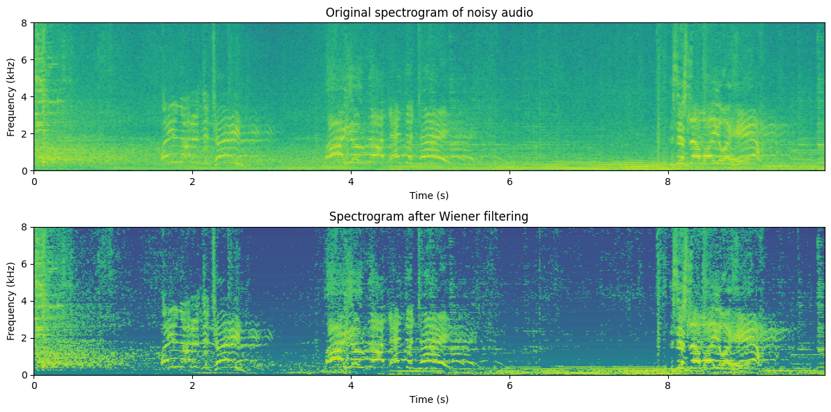
We find that noisefilling -type methods offer a compromise between the amount of noise removed and the amount of musical noise. Usually, we try to tune the parameter such that we are just above the level where musical noise is perceived since it is a non-natural distortion and therefore more annoying than an incomplete noise attenuation. However, closer tuning is dependent on application and preference.
11.1.4.2. Wiener filtering for vectors#
Above we considered the scalar case, or conversely, the case where we can treat components of a vector to be independent such that they can be equivalently treated as a collection of scalars. In some cases, however, we might be unable to find an uncorrelated representation of the signal or the corresponding whitening process could be unfeasibly complex or it can incur too much algorithmic delay. We then have to take into account the correlation between components.
Consider for example a desired signal \( x\in{\mathbb R}^{N \times1} \) , a noise signal \( v\in{\mathbb R}^{N \times1} \) and their additive sum, the observation \( y = x+v, \) from which we want to estimate the desired signal with a linear filter \( \hat x := a^H y. \) Following the MMSE derivation above, we set the derivative of the error energy expectation to zero
Where the covariance matrices are \( R_{xx} = E[xx^H] \) and \( R_{vv} = E[vv^H] \) , and we used the fact that \(x\) and \(v\) are uncorrelated \( E[xv^H]=0 \) . The solution is then clearly
where we for now assume that the inverse exists. This solution is clearly similar to the MMSE solution for the scalar case.
A central weakness of this approach is that it involves a matrix inversion, which is a computationally complex operation, such that online application is challenging. It furthermore requires that the covariance matrix \(R_{yy}\) is invertible (positive definite), which places constraints on the methods for estimating such covariances.
In any case, Wiener filtering is a convenient method, because it provides an analytical expression for an optimal solution in noise attenuation. It consequently has very well-documented properties and performance guarantees.
11.1.5. Masks, power spectra and temporal characteristics#
As seen above, we can attenuate noise if we have a good estimate of the noise energy. However, actually, both the spectral subtraction and Wiener filtering methods use models of the speech and noise energies. The models used above were rather heuristic; noise energy was assumed to be “known” and speech energy was defined as energy of observation minus noise energy. It is however not very difficult to make better models than that. Before going to improved models, note that we did not use speech and noise energies independently, but only their ratio. Now clearly the ratio of speech and noise is the signal-to-noise ratio (SNR) of that particular component. We thus obtain an estimate of the SNR of the whole spectrum. Conversely, we would need only the SNR of the spectrum to attenuate noise with the above methods. The SNR as a function of frequency and time is often referred to as a mask and in the following we will discuss some methods for generating such masks. It is however important to understand that mask-based methods are operating on the power (or magnitude) spectrum and thus do not include any models of the complex phase. Indeed, efforts have in general focused mostly on the power spectrum and much less on the phase. On one hand, the motivation is that characteristics of the power spectrum are much more important to perception than the phase (though the phase is also important), but on the other hand, the power spectrum is also much easier to work with than the phase. Therefore there has been both much more demand and supply of methods that treat the power spectrum.
To model speech signals, we can begin by looking at spectral envelopes, the high-level structure of the power spectrum. It is well-known that the phonetic information of speech lies primarily in the shape of the spectral envelope, and the lowest-frequency peaks of the envelope identify the vowels uniquely. In other words, the distribution of spectral energy varies smoothly across the frequencies. This is something we can model and use to estimate the spectral mask. Similarly, we know that phonemes vary slowly over time, which means that the envelope varies slowly over time. Thus, again, we can model envelope behavior over time to generate spectral masks.
A variation of such masks is known as binary masks, where we can set, for example, that the mask is 1 if speech energy is larger than noise energy, and 0 otherwise. Clearly, this is equivalent to thresholding the SNR at unity (which is equivalent to 0 dB), such that an SNR-mask can always be converted to a binary mask, but the reverse is not possible. The benefit of binary masks is that it simplifies some computations.
If we then want to attenuate noise in a particular frame of speech it is then useful to use as much of the surrounding data (context) as possible. For best quality, we can model, say, a second of the speech signal both before and after the target frame. Though this can improve the quality of the estimate, this has two clear negative consequences. First of all, including more data increases computational complexity. The level of acceptable complexity is highly dependent on the application. Secondly, if we look into future frames to process the current frame, then we have to have access to such data. In an online system, this means that we have to wait for the whole look-ahead data to arrive before processing, such that the overall system has a delay corresponding to the length of the look-ahead. We can extrapolate the current frame from past frames, but interpolating between past and future frames does give much better quality. The amount of acceptable delay is also an application-dependent question.
11.1.6. Machine learning methods#
By now, all state-of-the-art methods for noise attenuation are based on deep neural networks. The basic idea is that the neural network takes some features of the noisy speech signal as input and predicts the clean (noise-free) signal. The network is trained by inputting noisy signals and minimizing the difference between the predicted output and the clean signal.

One of the simplest possible approaches is to (simplified from [Valin, 2018])
use the magnitude spectrum of a single frame of speech as the input feature,
use a Gated Recurrent Unit (GRU) layer (24 dimensions) sandwiched between two linear layers,
the output is a mask that is multiplied with the noisy spectrum, to give the predicted spectrum, and
as a loss function, use the absolute difference of the decibel-power spectrum.

The training of this model is implemented elsewhere and here we include only the pretrained models. The performance is demonstrated below.
Show code cell source
import torch
import torchaudio
from frontend import PreProcessing, PostProcessing
class SimpleEnhancer(torch.nn.Module):
def __init__(
self,
spec_size = 241,
input_samplerate = 16000,
n_mels = 24,
smoothing = 0.7,
device = 'cpu',
):
super().__init__()
self.device = device
self.spec_size = spec_size
self.n_mels = n_mels
self.eval_state = False
self.smoothing = smoothing
self.melscale_transform = torchaudio.functional.melscale_fbanks(
self.spec_size,
f_min = 0,
f_max = input_samplerate / 2.0,
n_mels = n_mels,
sample_rate = input_samplerate,
norm = 'slaney',
)
self.melscale_transform = self.melscale_transform.to(device)
self.GRU = torch.nn.GRU(
input_size = n_mels,
hidden_size = 24,
device=device
)
self.dense_output = torch.nn.Sequential(
torch.nn.Linear(
self.GRU.hidden_size,
self.spec_size,
device = device),
torch.nn.Sigmoid()
)
def eval(self):
self.eval_state = True
return
def train(self):
self.eval_state = False
return
def forward(self, input_spec: torch.Tensor) -> torch.Tensor:
input_features = torch.matmul(
input_spec.abs()**2,
self.melscale_transform)
hidden,_ = self.GRU(input_features)
gains = self.dense_output(hidden)
if self.eval_state:
for k in range(gains.shape[-2]-1):
gains[...,k+1,:] = (
(1-self.smoothing)*gains[...,k+1,:] +
self.smoothing *gains[...,k,:] )
estimated_spec = input_spec * gains
return estimated_spec, gains
def oracle_gains(self, noisy_spec: torch.Tensor, clean_spec: torch.Tensor) -> torch.Tensor:
return (clean_spec.abs()/noisy_spec.abs().clamp(min=1e-6)).clamp(max=1)
class NoiseModelEnhancer(torch.nn.Module):
def __init__(
self,
input_samplerate = 16000,
spec_size = 241,
enhancer_size = 48,
noise_model_size = 24,
n_mels = 24,
smoothing = 0.2,
device = 'cpu'
):
super().__init__()
self.device = device
self.spec_size = spec_size
self.eval_state = False
self.smoothing = smoothing
self.melscale_transform = torchaudio.functional.melscale_fbanks(
self.spec_size,
f_min = 0,
f_max = input_samplerate / 2.0,
n_mels = n_mels,
sample_rate = input_samplerate,
norm = 'slaney',
)
self.melscale_transform = self.melscale_transform.to(device)
self.noise_model = torch.nn.GRU(
input_size = n_mels,
hidden_size = noise_model_size,
device=device
)
self.enhancer = torch.nn.GRU(
input_size = n_mels + noise_model_size,
hidden_size = enhancer_size,
device=device
)
self.dense_output = torch.nn.Sequential(
torch.nn.Linear(
self.enhancer.hidden_size,
self.spec_size,
device=device),
torch.nn.Sigmoid()
)
def eval(self):
self.eval_state = True
return
def train(self):
self.eval_state = False
return
def forward(self, input_spec: torch.Tensor) -> torch.Tensor:
input_features = torch.matmul(
input_spec.abs()**2,
self.melscale_transform)
noise_estimate,_ = self.noise_model(input_features)
enhancer_features = torch.cat((input_features, noise_estimate),dim=-1)
hidden,_ = self.enhancer(enhancer_features)
gains = self.dense_output(hidden)
if self.eval_state:
for k in range(gains.shape[-2]-1):
gains[...,k+1,:] = (
(1-self.smoothing)*gains[...,k+1,:] +
self.smoothing *gains[...,k,:] )
estimated_spec = input_spec * gains
return estimated_spec, gains
def oracle_gains(self, noisy_spec: torch.Tensor, clean_spec: torch.Tensor) -> torch.Tensor:
return (clean_spec.abs()/noisy_spec.abs().clamp(min=1e-6)).clamp(max=1)
class VADNoiseModelEnhancer(torch.nn.Module):
def __init__(
self,
spec_size = 241,
input_samplerate = 16000,
enhancer_size = 48,
noise_model_size = 24,
vad_model_size = 24,
n_mels = 24,
smoothing = 0.1,
device='cpu'
):
super().__init__()
self.device = device
self.spec_size = spec_size
self.n_mels = n_mels
self.eval_state = False
self.smoothing = smoothing
self.melscale_transform = torchaudio.functional.melscale_fbanks(
self.spec_size,
f_min = 0,
f_max = input_samplerate / 2.0,
n_mels = n_mels,
sample_rate = input_samplerate,
norm = 'slaney',
)
self.melscale_transform = self.melscale_transform.to(device)
self.VAD = torch.nn.GRU(
input_size = n_mels,
hidden_size = vad_model_size,
device=device
)
self.VAD_output = torch.nn.Linear(vad_model_size,1,device=device)
self.noise_model = torch.nn.GRU(
input_size = n_mels + vad_model_size,
hidden_size = noise_model_size,
device=device
)
self.enhancer = torch.nn.GRU(
input_size = n_mels + noise_model_size + vad_model_size,
hidden_size = enhancer_size,
device=device
)
self.dense_output = torch.nn.Sequential(
torch.nn.Linear(
self.enhancer.hidden_size,
self.spec_size,
device=device),
torch.nn.Sigmoid()
)
def eval(self):
self.eval_state = True
return
def train(self):
self.eval_state = False
return
def forward(self, input_spec: torch.Tensor) -> torch.Tensor:
input_features = torch.matmul(
input_spec.abs()**2,
self.melscale_transform)
vad_estimate,_ = self.VAD(input_features)
vad_output = self.VAD_output(vad_estimate)
noise_estimate,_ = self.noise_model(torch.cat(
(input_features,
vad_estimate),
dim=-1))
hidden,_ = self.enhancer(torch.cat(
(input_features,
noise_estimate,
vad_estimate),
dim=-1))
gains = self.dense_output(hidden)
if self.eval_state:
for k in range(gains.shape[-2]-1):
gains[...,k+1,:] = (
(1-self.smoothing)*gains[...,k+1,:] +
self.smoothing *gains[...,k,:] )
estimated_spec = input_spec * gains
return estimated_spec, gains
def oracle_gains(self, noisy_spec: torch.Tensor, clean_spec: torch.Tensor) -> torch.Tensor:
return (clean_spec.abs()/noisy_spec.abs().clamp(min=1e-6)).clamp(max=1)
Show code cell source
target_rate = 16000
# read from storage
device = 'cpu'
fs, data = wavfile.read(filename)
print(f"Input sample rate {fs} Hz")
data_torch = torch.Tensor(data[:],device=device)
preprocessor = PreProcessing(input_samplerate=fs)
postprocessor = PostProcessing(output_samplerate=fs)
enhancer_state_dict = torch.load('SimpleEnhancer_MelLoss.pt')
enhancer = SimpleEnhancer(spec_size = preprocessor.output_size,
input_samplerate = target_rate,
device=device)
enhancer.load_state_dict(enhancer_state_dict)
enhancer.eval()
Input sample rate 44100 Hz
noisy_spectrogram = preprocessor(data_torch)
noisy_audio = postprocessor(noisy_spectrogram)
enhanced_spectrogram,_ = enhancer(noisy_spectrogram)
enhanced_audio = postprocessor(enhanced_spectrogram)
enhanced_audio = enhanced_audio*noisy_audio.std()/enhanced_audio.std()
Show code cell source
length_in_s = len(noisy_audio)/fs
plt.figure(figsize=(5,6))
plt.subplot(211)
plt.imshow(noisy_spectrogram.abs().log().T.numpy(),
origin='lower',aspect='auto',
extent=[0, length_in_s, 0, 16000/2000])
plt.axis([0, length_in_s, 0, 8])
plt.xlabel('Time (s)')
plt.ylabel('Frequency (kHz)');
plt.title('Noisy')
plt.subplot(212)
plt.imshow(enhanced_spectrogram.abs().log().T.detach().numpy(),
origin='lower',aspect='auto',
extent=[0, length_in_s, 0, 16000/2000])
plt.axis([0, length_in_s, 0, 8])
plt.xlabel('Time (s)')
plt.ylabel('Frequency (kHz)');
plt.title('Simple DNN Estimate')
plt.tight_layout()
plt.show()
import IPython
IPython.display.display(IPython.display.Audio(noisy_audio,rate=int(fs)))
IPython.display.display(IPython.display.Audio(enhanced_audio.detach().numpy(),rate=int(fs)))
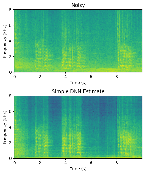
Though this is certainly not perfect, it is rather desent with such a simple model. The difficulty is that it has to retain both a speech model and noise model in its 24-dimensional GRU. A straightforward way is thus to separate the noise model into itse own layer, and feed that to the enhancer-module.

Show code cell source
# read from storage
fs, data = wavfile.read(filename)
data_torch = torch.Tensor(data[:],device=device)
enhancer_state_dict = torch.load('NoiseModelEnhancer_MelLoss.pt')
enhancer = NoiseModelEnhancer(spec_size = preprocessor.output_size,
input_samplerate = target_rate,
device=device)
enhancer.load_state_dict(enhancer_state_dict)
enhancer.eval()
noisy_spectrogram = preprocessor(data_torch)
noisy_audio = postprocessor(noisy_spectrogram)
enhanced_spectrogram,_ = enhancer(noisy_spectrogram)
enhanced_audio = postprocessor(enhanced_spectrogram)
enhanced_audio = enhanced_audio*noisy_audio.std()/enhanced_audio.std()
Show code cell source
length_in_s = len(noisy_audio)/fs
plt.figure(figsize=(5,6))
plt.subplot(211)
plt.imshow(noisy_spectrogram.abs().log().T.numpy(),
origin='lower',aspect='auto',
extent=[0, length_in_s, 0, 16000/2000])
plt.axis([0, length_in_s, 0, 8])
plt.xlabel('Time (s)')
plt.ylabel('Frequency (kHz)');
plt.title('Noisy')
plt.subplot(212)
plt.imshow(enhanced_spectrogram.abs().log().T.detach().numpy(),
origin='lower',aspect='auto',
extent=[0, length_in_s, 0, 16000/2000])
plt.axis([0, length_in_s, 0, 8])
plt.xlabel('Time (s)')
plt.ylabel('Frequency (kHz)');
plt.title('DNN with Noise Model Estimate')
plt.tight_layout()
plt.show()
import IPython
IPython.display.display(IPython.display.Audio(noisy_audio,rate=int(fs)))
IPython.display.display(IPython.display.Audio(enhanced_audio.detach().numpy(),rate=int(fs)))
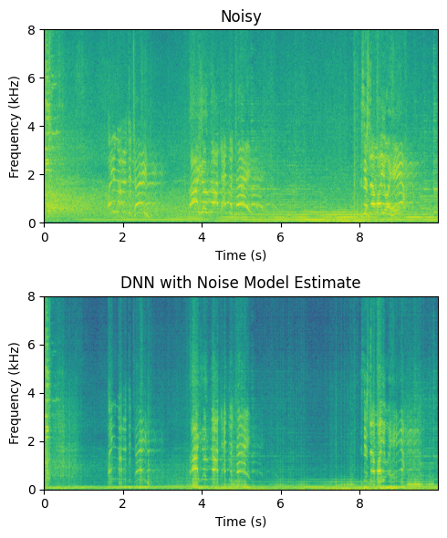
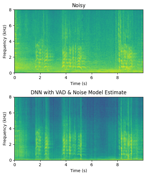
We can further improve the result by integrating a voice activity detector (VAD) into the pipeline, such that the VAD output is fed into the noise model and enhancer modules.

Show code cell source
# read from storage
fs, data = wavfile.read(filename)
data_torch = torch.Tensor(data[:],device=device)
enhancer_state_dict = torch.load('VADNoiseModelEnhancer_MelLoss.pt')
enhancer = VADNoiseModelEnhancer(spec_size = preprocessor.output_size,
input_samplerate = target_rate,
device=device)
enhancer.load_state_dict(enhancer_state_dict)
enhancer.eval()
noisy_spectrogram = preprocessor(data_torch)
noisy_audio = postprocessor(noisy_spectrogram)
enhanced_spectrogram,_ = enhancer(noisy_spectrogram)
enhanced_audio = postprocessor(enhanced_spectrogram)
enhanced_audio = enhanced_audio*noisy_audio.std()/enhanced_audio.std()
Show code cell source
length_in_s = len(noisy_audio)/fs
plt.figure(figsize=(5,6))
plt.subplot(211)
plt.imshow(noisy_spectrogram.abs().log().T.numpy(),
origin='lower',aspect='auto',
extent=[0, length_in_s, 0, 16000/2000])
plt.axis([0, length_in_s, 0, 8])
plt.xlabel('Time (s)')
plt.ylabel('Frequency (kHz)');
plt.title('Noisy')
plt.subplot(212)
plt.imshow(enhanced_spectrogram.abs().log().T.detach().numpy(),
origin='lower',aspect='auto',
extent=[0, length_in_s, 0, 16000/2000])
plt.axis([0, length_in_s, 0, 8])
plt.xlabel('Time (s)')
plt.ylabel('Frequency (kHz)');
plt.title('DNN with VAD & Noise Model Estimate')
plt.tight_layout()
plt.show()
import IPython
IPython.display.display(IPython.display.Audio(noisy_audio,rate=int(fs)))
IPython.display.display(IPython.display.Audio(enhanced_audio.detach().numpy(),rate=int(fs)))
11.1.6.1. Pretrained model: SpeechBrain#
From SpeechBrain Basics
SpeechBrain is an open-source all-in-one speech toolkit based on PyTorch. It is designed to make the research and development of speech technology easier. Alongside with our documentation this tutorial will provide you all the very basic elements needed to start using SpeechBrain for your projects.
It contains also a standard implementation of speech enhancement. For more information, see Speech Enhancement From Scratch.
from speechbrain.inference.enhancement import SpectralMaskEnhancement
enhancer = SpectralMaskEnhancement.from_hparams(
source="speechbrain/metricgan-plus-voicebank",
savedir='.',
)
enhanced_audio_speechbrain = enhancer.enhance_file("sounds/enhancement_test_16k.wav")
Show code cell source
fs, data = wavfile.read("sounds/enhancement_test_16k.wav")
data_torch = torch.Tensor(data[:],device=device)
preprocessor16 = PreProcessing(input_samplerate=fs)
noisy_spectrogram = preprocessor16(data_torch)
enhanced_spectrogram_speechbrain = preprocessor16(enhanced_audio_speechbrain)
length_in_s = len(data)/fs
plt.figure(figsize=(5,6))
plt.subplot(211)
plt.imshow(noisy_spectrogram.abs().log().T.numpy(),
origin='lower',aspect='auto',
extent=[0, length_in_s, 0, 16000/2000])
plt.axis([0, length_in_s, 0, 8])
plt.xlabel('Time (s)')
plt.ylabel('Frequency (kHz)');
plt.title('Noisy')
plt.subplot(212)
plt.imshow(enhanced_spectrogram_speechbrain.abs().log().T.detach().numpy(),
origin='lower',aspect='auto',
extent=[0, length_in_s, 0, 16000/2000])
plt.axis([0, length_in_s, 0, 8])
plt.xlabel('Time (s)')
plt.ylabel('Frequency (kHz)');
plt.title('Enhanced with SpeechBrain DNN')
plt.tight_layout()
plt.show()
import IPython
IPython.display.display(IPython.display.Audio(data,rate=int(fs)))
IPython.display.display(IPython.display.Audio(enhanced_audio_speechbrain.detach().numpy(),rate=int(fs)))
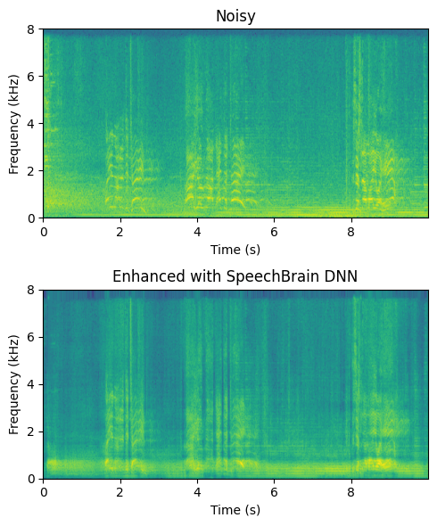
The character of this output is rather different than previous examples. It is more smooth, but more of the background music is preserved in the low frequency and speech sounds metallic and muffled.
11.1.6.2. Datasets and training#
The first choice in designing machine learning methods for noise attenuation and other speech enhancement tasks is the overall systems architecture. The application is usually simply a neural network that takes noisy speech as input and outputs an estimate of the clean speech. A natural choice would then be to train the network with a large database of noisy speech samples and minimize the distance of the output to the clean speech signal. Since we assume that noise is additive, we can create synthetic samples by adding noise to speech. By varying the intensity (volume) of the noise samples, we can further choose the signal-to-noise ratio of the noise samples. With reasonable size databases of speech and noise, we thus get a practically infinite number of unique noisy samples such that we can make even a large neural network converge.
A weakness of this model however is that even if the database is thus large, it has only a limited number of unique noises and unique speakers. There is no easy way of getting assurance that unseen noises and speakers will be enhanced effectively. What if we receive a noisy sample where a 3-year-old child talks with annoying vuvuzelas playing in the background? If our database contained only adult speakers and did not contain vuvuzela sounds, then we cannot know whether our enhancement is effective on the noisy sample.
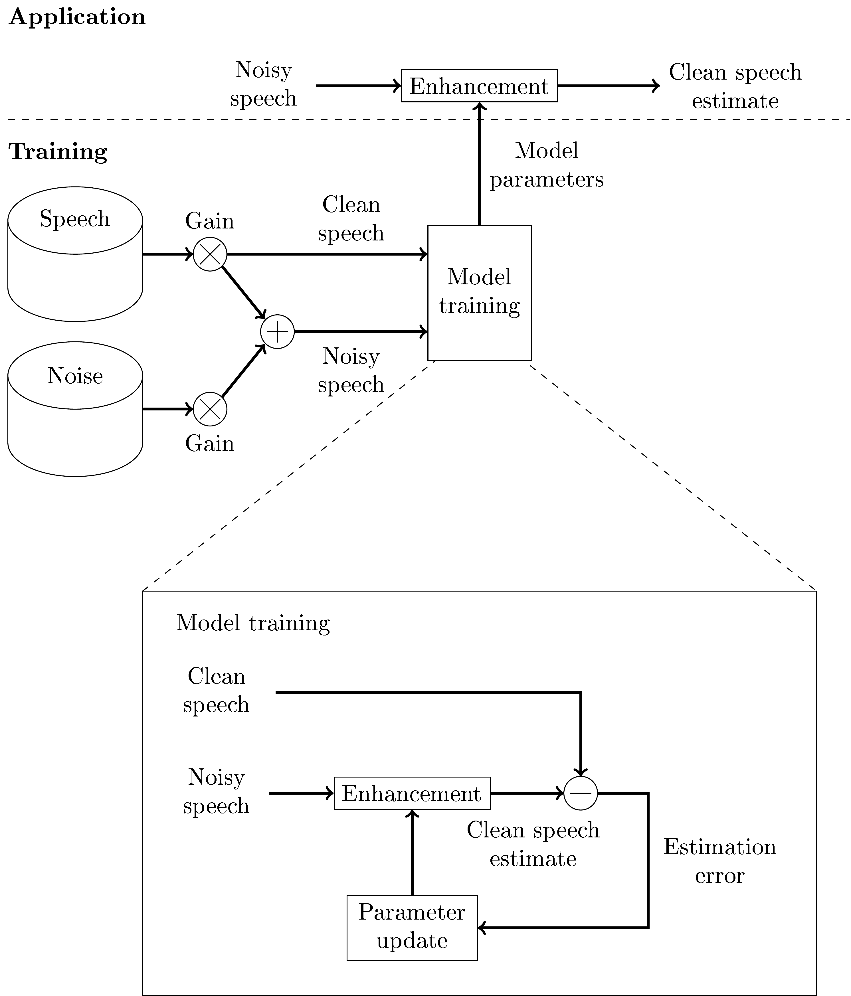 Machine learning configuration for speech enhancement with noisy and target clean speech signal.
To overcome the problem of inadequate noise databases, we can take an adversarial approach, where we have a generative network that generates noises and an enhancement network that attenuates noises that corrupt speech. This approach is known as a generative adversarial network (GAN). We then have two optimization tasks;
To optimize the enhancement network (minimize estimation error) to remove the noise generated by the generative network and
to optimize the generative network (maximize estimation error) to generate noises that the enhancement network is unable to remove.
These two tasks are adversarial in the sense that they work against each other. In practical application we would use only the enhancement network, so the generative network is used only in training.
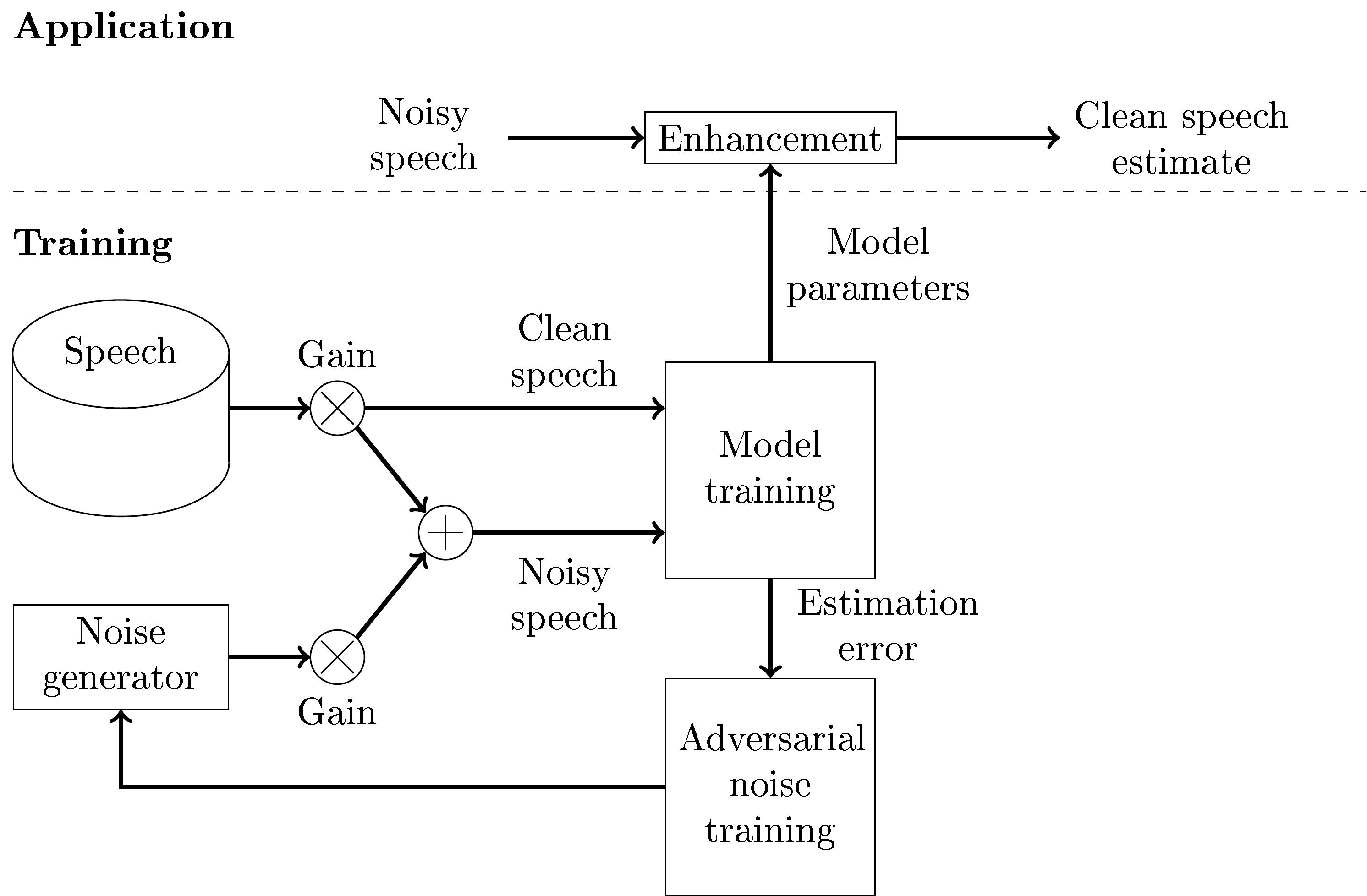 Application and training with a generative adversarial network (GAN) structure for speech enhancement.
11.1.7. References#
For a recent review of speech enhancement, see [Zheng et al., 2023].
Jacob Benesty, M Mohan Sondhi, Yiteng Huang, and others. Springer handbook of speech processing. Volume 1. Springer, 2008. URL: https://doi.org/10.1007/978-3-540-49127-9.
Steven Boll. Suppression of acoustic noise in speech using spectral subtraction. IEEE Transactions on acoustics, speech, and signal processing, 27(2):113 – 120, 1979. URL: https://doi.org/10.1109/TASSP.1979.1163209.
Rainer Martin. Noise power spectral density estimation based on optimal smoothing and minimum statistics. IEEE Transactions on speech and audio processing, 9(5):504 – 512, 2001. URL: https://doi.org/10.1109/89.928915.
Jean-Marc Valin. A hybrid dsp/deep learning approach to real-time full-band speech enhancement. In 2018 IEEE 20th international workshop on multimedia signal processing (MMSP), 1–5. IEEE, 2018. URL: https://doi.org/10.1109/MMSP.2018.8547084.
Chengshi Zheng, Huiyong Zhang, Wenzhe Liu, Xiaoxue Luo, Andong Li, Xiaodong Li, and Brian CJ Moore. Sixty years of frequency-domain monaural speech enhancement: from traditional to deep learning methods. Trends in Hearing, 2023. URL: https://doi.org/10.1177/23312165231209913.