5.6. Neural networks#
5.6.1. Introduction#
An Artificial Neural Network (ANN) is a mathematical model that tries to simulate the structure and functionalities of biological neural networks. Basic building block of every artificial neural network is artificial neuron, that is, a simple mathematical model (function). Artificial neuron is a basic building block of every artificial neural network. Its design and functionalities are derived from observation of a biological neuron that is basic building block of biological neural networks (systems) which includes the brain, spinal cord and peripheral ganglia.
Computational modelling using neural networks was started in the 1940’s and has gone through several waves of innovation and subsequent decline. The recent boom of deep neural networks (DNNs) - which roughly means that the network has more layers of non-linearities than previous models - happened probably due to the increase in available computational power and availability of large data-sets. It has fuelled a flurry of incremental innovation in all directions, and in many modelling tasks, deep neural networks currently give much better results than any competing method.
Despite its successes, application of DNNs in speech processing does not come without its fair share of problems. For example,
Training DNNs for a specific task on a particular set of data often does not increase our understanding of the problem. It is a black box. How are we to know whether the model is reliable? A trained speech recognizer on a language A does not teach much about speech recognition for language B (though the process of designing a recognizers does teach us about languages).
Training of DNNs is sensitive to the data on which it is trained on. Models can for example be susceptible to hidden biases, such that performance degrades for particular under-represented groups of people.
A trained DNN is “a solution” to a particular problem, but it does not directly give us information about how good of a solution it is. For example, if a data-set represents a circle in the 2D-plane, then it is possible to accurately model that data-set with a neural network where the non-linearities are sigmoids. The neural network just has to be large enough and it can do the job. However, the network is then several orders of magnitude more complex than the equation of the circle. That is, though training of the network was successful, and the model is relatively accurate, it gives no indication if the complexity of the network is of similar scale as the complexity of the problem.
To combat such problems, a recent trend in model design has been to return to classical design paradigms, where models are based on thorough understanding of the problem. The parameters of such models are then trained using methods from machine learning.
5.6.2. Network structures#
Neural networks are, in principle, built from simple building blocks, where the most common type of building block is
where x is an input vector, matrix A and vector b are constants, f is a non-linear function such as the element-wise sigmoid, and y is the output. This is often referred to as a layer. Layers can then be stacked after each other such that, for example, a three layer network would be
5.6.2.1. Deep Neural Networks (DNNs)#
Deep Neural Network (DNNs) are an artificial neural network (ANN) with multiple layers between the input and output layers. Many experts define deep neural networks as networks that have an input layer, an output layer and at least one hidden layer in between. Each layer performs specific types of sorting and ordering in a process that some refer to as “feature hierarchy.” One of the key uses of these sophisticated neural networks is dealing with unlabeled or unstructured data. The phrase “deep learning” is also used to describe these deep neural networks, as deep learning represents a specific form of machine learning where technologies using aspects of artificial intelligence seek to classify and order information in ways that go beyond simple input/output protocols.
5.6.2.2. Basics of Neural Networks#
Neurons: It forms the basic structure of a neural network. When we get the information, we process it and then we generate an output. Similarly, a neuron receives an input, processes it and generates an output which is either sent to other neurons for further processing or it is the final output.
Weights: When an input enters a neuron, it is multiplied by a weight. Initially, the weights are initialized and they are updated during the model training process. When the training is over, the neural network assigns a higher weight value to the input it considers more important as compared to the ones which are considered less important.
Bias: In addition to the weights, another linear component is applied to the input, called as the bias. It is added to the result of weight multiplication to the input. The bias is basically added to change the range of the weight multiplied input.
5.6.2.3. Activation Functions:#
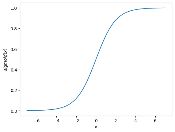
Sigmoid: It allows a reduction in extreme or atypical values in valid data without eliminating them: it converts independent variables of almost infinite range into simple probabilities between 0 and 1. Most of its output will be very close to the extremes of 0 or 1. $\( sigmoid(x) = \frac{1}{1+e^{-x}} \)$
import numpy as np
import matplotlib.pyplot as plt

x = np.linspace(-7,7,100)
plt.plot(x, 1./(1. + np.exp(-x)))
plt.xlabel('$x$')
plt.ylabel('$sigmoid(x)$')
plt.show()
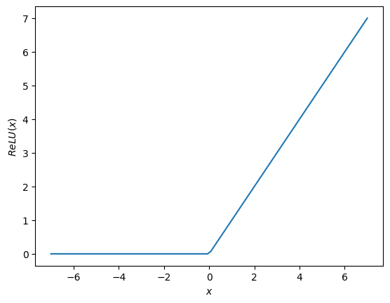
ReLU(Rectified Linear Unit): It has output 0 if the input is less than 0, and raw output otherwise. That is, if the input is greater than 0, the output is equal to the input. The operation of ReLU is closer to the way our biological neurons work. $\( ReLU(x) = \max(x,0) = \begin{cases} x, & x>0\\ 0, & \text{otherwise}.\end{cases} \)$
import numpy as np
import matplotlib.pyplot as plt

x = np.linspace(-7,7,100)
plt.plot(x, (x>0)*x)
plt.xlabel('$x$')
plt.ylabel('$ReLU(x)$')
plt.show()
Softmax: A modification of the regular \(\max\) over a vector, such that it has a continuous derivative everywhere. That is, it maps the output to the range \([0,1]\) and simultaenously ensures that the total sum is 1. The output of Softmax is therefore a probability distribution. $\( SoftMax (\mathbf {x_k} )=\frac {e^{x_k}}{\sum _{j=1}^{K}e^{x_j}}.\)$
Input / Output / Hidden Layer : The input layer receives the input and is the first layer of the network. The output layer is the one which generates the output and is the final layer of the network. The processing layers are the hidden layers within the network. These hidden layers are the ones which perform specific tasks on the incoming data and pass on the output generated by them to the next layer. The input and output layers are the ones visible to us, while are the intermediate layers are hidden.
MLP (Multi Layer perceptron): In the simplest network, we would have an input layer, a hidden layer and an output layer. Each layer has multiple neurons and all the neurons in each layer are connected to all the neurons in the next layer. These networks can also be called as fully connected networks.
Cost or loss function: When we train a network, its main objective is to to predict the output as close as possible to the actual value. Hence, the cost/loss function is used to measure this accuracy. The cost or loss function penalizes the network when it makes errors. The main objective while running the network is to increase the prediction accuracy and to reduce the error, thus minimizing the cost function.
Gradient Descent: It is an optimization algorithm used to minimize some function by iteratively moving in the direction of steepest descent as defined by the negative of the gradient.
Learning Rate: The learning rate is a hyperparameter that controls how much to change the model in response to the estimated error each time the model weights are updated. Choosing the learning rate is challenging as a value too small may result in a long training process that could get stuck, whereas a value too large may result in learning a sub-optimal set of weights too fast or an unstable training process. The learning rate may be the most important hyperparameter when configuring neural network. Therefore, it is important to know how to investigate the effects of the learning rate on model performance and to build an intuition about the dynamics of the learning rate on model behavior.
Backpropagation: When we define a neural network, we assign random weights and bias values to our nodes. Once we have received the output for a single iteration, we can calculate the error of the network. This error is then fed back to the network along with the gradient of the cost function to update the weights of the network. These weights are then updated so that the errors in the subsequent iterations is reduced. This updating of weights using the gradient of the cost function is known as back-propagation. In back-propagation the movement of the network is backwards, the error along with the gradient flows back from the out layer through the hidden layers and the weights are updated.
Batches: While training a neural network, instead of sending the entire input in one go, we divide in input into several chunks of equal size randomly. Training the data on batches makes the model more generalized as compared to the model built when the entire data set is fed to the network in one go.
Epochs: An epoch is is a single training iteration of all batches in both forward and back propagation. Thus, 1 epoch is a single forward and backward pass of the entire input data. Although it is highly likely that more number of epochs would show higher accuracy of the network, it would also take longer for the network to converge. You should also take into account that if the number of epochs are too high, the network might over-fit.
Dropout: It is a regularization technique to prevent over-fitting of the network. While training, a number of neurons in the hidden layer are randomly dropped.
Batch Normalization: It normalizes the input layer by adjusting and scaling the activations. For example, if we have features from 0 to 1 and some from 1 to 1000, we should normalize them to speed up learning.
Classification of Neural Networks
Shallow neural network: It has only one hidden layer between the input and output.
Deep neural network: it has more than one layer.
Types of Deep Learning Networks

Feed forward neural networks: They are artificial neural networks where the connections between units do not form a cycle. Feedforward neural networks were the first type of artificial neural network invented and are simpler than their counterpart, recurrent neural networks (see below ). They are called feedforward because information only travels forward in the network. Firstly, it goes through the input nodes, then through the hidden nodes and finally through the output nodes.
5.6.2.4. Convolutional neural networks#
CNN was first proposed by [1]. It has first been successfully used by [2] for handwritten digit classification problem. It is currently the most popular neural network model being used for image classification problem. The advantages of CNNs over DNNs include CNNs are highly optimized for processing 2D and 3D images, and are effective to learn and extract abstractions of 2D features. In addition to these, CNNs have significantly fewer parameters than a fully connected network of similar size.
Figure 4.1. shows the overall architecture of CNNs. CNNs consists mainly of two parts: feature extractors and classifier. In the feature extraction module, each layer of the network receives the output from its immediate previous layer as its input and passes its output as the input to the next layer. The CNN architecture mainly consists of three types of layers: convolution, pooling, and classification.
Figure 4.1. An overall architecture of the Convolutional Neural Network.
The main layers in Convolutional Neural Networks are:
Convolutional layer: A “filter” passes over the image, scanning a few pixels at a time and creating a feature map that predicts the class to which each feature belongs. Thus, in this layer, feature maps from previous layers are convolved with learnable kernels. The output of the kernels goes through a linear or non-linear activation function, such as sigmoid, hyperbolic tangent, Softmax, rectified linear, and identity functions) to form the output feature maps. Each of the output feature maps can be combined with more than one input feature map.
Pooling layer: It reduces the amount of information in each feature obtained in the convolutional layer while maintaining the most important information (there are usually several rounds of convolution and pooling).
Fully connected input layer (flatten): It takes the output of the previous layers, “flattens” them and turns them into a single vector that can be an input for the next stage.
The first fully connected layer: It takes the inputs from the feature analysis and applies weights to predict the correct label.
Fully connected output layer: It gives the final probabilities for each label.
Higher-level features are derived from features propagated from lower level layers. As the features propagate to the highest layer or level, the dimensions of features are reduced based on the size of the kernel for the convolution and pooling operations respectively. However, the number of feature maps usually increase for representing better features of the input images for ensuring classification accuracy. The output of the last layer of the CNN is used as the input to a fully connected network. Feed-forward neural networks are used as the classification layer since they provide better performance.
Figure 4.2 Popular CNN architectures. The Figure is taken from https://www.aismartz.com/blog/cnn-architectures/.
Applications of CNNs:
Image Processing and Computer Vision: CNNs have been successfully used in different image classification tasks [7–11].
Speech Processing: CNNs have been successfully used in different speech processing applications such as speech enhancement [8] and audio tagging [9].
Medical Imaging: CNNs have also been widely used in different medical image processing including classification, detection, and segmentation tasks [10].
Training Techniques
Sub-Sampling Layer or Pooling Layer: Two different techniques have been used for the implementation of deep networks in the sub-sampling or pooling layer: average and max-pooling. While the average Pooling calculate the average value for each patch on the feature map, the max pooling calculate the maximum value for each patch of the feature map.
Padding: It adds extra layer of zeros across the images so that the output image has the same size as the input.
Data Augmentation: It is the addition of new data derived from the given data. This might prove to be beneficial for prediction. It includes rotation, shearing, zooming, cCropping, flipping and changing the brightness level.
Note that the performance of CNNs depends heavily on multiple hyperparameters: number of layers, number of feature maps in each layer, the use of dropouts, batch normalization, etc. Thus, it’s important that you should first fine-tune the model hyperparameters by conducting lots of experiments. Once you find the right set of hyperparameters, you need to train the model for a number of epochs.
5.6.2.5. Recurrent neural networks (RNNs)#
Topics to be covered:
Basics of RNNs
Vanishing and exploding gradient problem
Long short-term memory (LSTM)
Basics of RNNs
The standard feedforward neural networks (i.e,, DNNs and CNNs) are function generators associating appropriate output to input. However, certain types of data are serial in nature. A recurrent neural network (RNN) processes sequences such as stock prices, sentences one element at a time while retaining a memory (called a state) of what has come previously in the sequence. Recurrent means the output at the current time step becomes the input to the next time step. At each element of the sequence, the model considers not just the current input, but what it remembers about the preceding elements. This memory allows the network to learn long-term dependencies in a sequence which means it can take the entire context into account when making a prediction such as predicting the next word in a sentence. A RNN is designed to mimic the human way of processing sequences: we consider the entire sentence when we form a response instead of words by themselves. For example, consider the following sentence:
“The concert was boring for the first few minutes but then was terribly exciting.”
A machine learning model that considers the words in isolation would probably conclude this sentence is negative. An RNN by contrast should be able to see the words “but” and “terribly exciting” and realize that the sentence turns from negative to positive because it has looked at the entire sequence. Reading a whole sequence gives us a context for processing its meaning, a concept encoded in recurrent neural networks.
Figure 4.3 General form of RNN
The left part of Figure 4.3 shows that the input-output relation of a standard neural network is altered so that the output is fed into the input. But, the right part of Figure 4.3 shows that the scheme unwrapped through time. The input is the serial data \( (x_1,........,x_T) \) and the output is \( (o_1,........,o_T) \) . The output of a neural network is fed into the next constituent neural network in the next stage as part of the input. So the output \( o_t \) depends on all the inputs \( (x_1,........,x_T) \) . It may be the case that it is not a good idea to make the output \( o_1 \)
dependent only on \( x_1 \) . In fact \( o_1 \) itself should be produced in context.
RNNs can be used in different applications such as machine translation, speech recognition, generating image descriptions, video tagging, and language modeling.
Advantages of Recurrent Neural Network
An RNN remembers each and every information through time. It is useful in time series prediction only because of the feature to remember previous inputs as well. This is called Long Short Term Memory.
Recurrent neural network are even used with convolutional layers to extend the effective pixel neighborhood.
Disadvantages of Recurrent Neural Network
Gradient vanishing and exploding problems.
Training an RNN is a very difficult task.
It cannot process very long sequences if using tanh or relu as an activation function.
Vanishing and exploding gradient problem
RNNs are very hard to train. Let us see the reason. The term \( \frac{\partial E}{\partial h^l} \) used in backpropagation algorithm is a product of a long chain of matrices: \( \left( \frac {\partial E}{\partial h^l} \right ) = \left ( \frac {\partial z^{l+1}}{\partial h^l} \right ) \left ( \frac {\partial h^{l+1}}{\partial z^{l+1}} \right )...\left ( \frac {\partial h^l}{\partial z^L} \right ) \left ( \frac {\partial E}{\partial h^L} \right ), \) For the input \( x=h^0 \) , this chain is the longest. If the activation function \( sigmoid(t) \) is the sigmoid function \( sigmoid(t) = \frac{1}{1+e^{-t}} \) its derivative is \( sigmoid'(t) = \frac{e^t} { \left( 1 + e^t \right ) ^2 } \) which gets very small so that it practically vanishes except at a small interval near 0. It is one of the reasons why people ReLU activation function is prefered. But it is not a solution, as negative input values also kill the gradient and make it stay there. Even if one avoids such an outright vanishing gradient problem, the long matrix multiplication in general may make the gradient vanish or explode. This kind of problem gets even more aggravated in the case of RNNs, since RNNs normally require long chain of backpropagation not only through the layers of neural networks of constituent cells but also across the different cells. Hence, RNNs are difficult to train.
Long short-term memory (LSTM)
The Long Short-Term Memory (LSTM) was first proposed by Hochreiter and Schmidhuber [10] as a solution to the vanishing gradients problem. But it did not attract much attention until people realized it indeed provides a good solution to the vanishing and exploding gradient problem of RNN as described above. We will only describe the architecture of its cell. There are many variations in the cell architecture, but we present only the basics.
At the heart of an RNN is a layer made of memory cells. The most popular cell at the moment is the Long Short-Term Memory (LSTM) which maintains a cell state as well as a carry for ensuring that the signal (information in the form of a gradient) is not lost as the sequence is processed. At each time step the LSTM considers the current word, the carry, and the cell state. The LSTM has 3 different gates and weight vectors: there is a “forget” gate for discarding irrelevant information; an “input” gate for handling the current input, and an “output” gate for producing predictions at each time step. However, as Chollet points out, it is fruitless trying to assign specific meanings to each of the elements in the cell.

Figure 4.4. Structure of LSTM cell
The structure of LSTM is shown in Figure 4.4 . The input vector is \( x_t \) . The cell state denoted by \( c_{t-1} \) and the hidden state \( h_{t-1} \) are fed into the LSTM cell and \( c_t \) and \( h_t \) are fed into the next cell. Internally, it has four states: \( i_t \) (input), \( f_t \) (forget), \( o_t \) (output), and \( g_t \) . The forget state \( f_t \) is obtained as a sigmoid output of a network with \( x_t \) and \( h_{t-1} \) fed into it as inputs. Since \( f_t \) is a sigmoid output, each element in it has a value between 0 and 1. If it is close to 0, it erases \( c_{t-1} \) by multiplication; if it is close to 1, it keeps \( c_{t-1} \) by multiplication. Thus, \( f_t \) is given the name ”forget state” because of this property, The input state \( i_t \) and the output state \( o_t \) are obtained by using (1) and (3), respectively. The state \( g_t \) is also obtained similarly except that it is an output of the form tanh . This gives the \( \pm \) sign. The product it \( \\otimes \) gt is then added to \( c_t \) , and this gives new information to the cell state. The hidden state ht is obtained as in (6), and the cell output \( y_t \) is the same as \( h_t \) . The whole scheme is depicted in Figure 4.4.
5.6.3. References:#
[1] Fukushima, K. Neocognitron: A hierarchical neural network capable of visual pattern recognition. Neural Netw. 1988, 1, 119–130.
[2] LeCun, Y.; Bottou, L.; Bengio, Y.; Haffner, P. Gradient-based learning applied to document recognition. Proc. IEEE 1998, 86, 2278–2324.
[3] Krizhevsky, A.; Sutskever, I.; Hinton, G.E. Imagenet classification with deep convolutional neural networks. In Proceedings of the 25th International Conference on Neural Information Processing Systems, Lake Tahoe, NV, USA, 3–6 December 2012; pp. 1106–1114.
[4] Zeiler, M.D.; Fergus, R. Visualizing and understanding convolutional networks. arXiv 2013, arXiv:1311.2901.
[5] Simonyan, K.; Zisserman, A. deep convolutional networks for large-scale image recognition. arXiv 2014, arXiv:1409.1556.
[6] Szegedy, C.; Liu, W.; Jia, Y.; Sermanet, P.; Reed, S.; Anguelov, D.; Erhan, D.; Vanhoucke, V.; Rabinovich, A. Going deeper with convolutions. In Proceedings of the IEEE Conference on Computer Vision and Pattern Recognition, Boston, MA, USA, 7–12 June 2015; pp. 1–9.
[7] He, K.; Zhang, X.; Ren, S.; Sun, J. Deep residual learning for image recognition. In Proceedings of the IEEE Conference on Computer Vision and Pattern Recognition, Las Vegas, NV, USA, 27–30 June 2016; pp. 770– 778.
[8] Hou, J.-C.; Wang, S.; Lai, Y.; Tsao, Y.; Chang, H.; Wang, H. Audio-Visual Speech Enhancement Using Multimodal Deep Convolutional Neural Networks. arXiv 2017, arXiv:1703.10893.
[9] Xu, Y.; Kong, Q.; Huang, Q.; Wang, W.; Plumbley, M.D. Convolutional gated recurrent neural network incorporating spatial features for audio tagging. In Proceedings of the 2017 International Joint Conference on Neural Networks (IJCNN), Anchorage, AK, USA, 14–19 May 2017; pp. 3461–3466.
[10] Hochreiter, S., Schmidhuber, J., Courville, A., Long short-term memory, Neural Computation 9(8):1735-80 (1997)