5.2. Linear regression

5.2.1. Problem definition

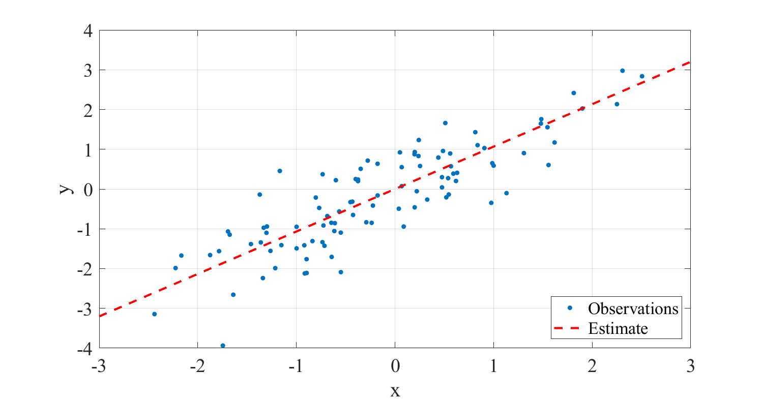
In speech processing and elsewhere, a frequently appearing task is to make a prediction of an unknown vector y from available observation vectors x. Specifically, we want to have an estimate \( \hat y = f(x) \) such that \( \hat y \approx y. \) In particular, we will focus on linear estimates where \( \hat y=f(x):=A^T x, \) and where A is a matrix of parameters. The figure on the right illustrates a linear model, where the input sample pairs (x,y) are modelled by a linear model \( \hat y \approx ax. \)

5.2.2. The minimum mean square estimate (MMSE)

Suppose we want to minimise the squared error of our estimate on average. The estimation error is \( e=y-\hat y \) and the squared error is the \(L_{2}\)-norm of the error, that is, \( \left\|e\right\|^2 = e^T e \) and its mean can be written as the expectation \( E\left[\left\|e\right\|^2\right] = E\left[\left\|y-\hat y\right\|^2\right] = E\left[\left\|y-A^T x\right\|^2\right]. \) Formally, the minimum mean square problem can then be written as

\[ \min_A\, E\left[\left\|y-A^T x\right\|^2\right]. \]

This can in generally not be directly implemented because we have the abstract expectation-operation in the middle.

(Advanced derivation begins) To get a computational model, first note that the error expectation can be written in terms of the mean of a sample of vector e_{k} as

\[ E\left[\left\|e\right\|^2\right] \approx \frac1N \sum_{k=1}^N \left\|e_k\right\|^2 = \frac1N {\mathrm{tr}}(E^T E), \]

where \( E=\left[e_1,\,e_2,\dotsc,e_N\right] \) and tr() is the matrix trace. To minimize the error energy expectation, we can then set its derivative to zero

\[ 0 = \frac{\partial}{\partial A} \frac1N {\mathrm{tr}}(E^T E) = \frac1N\frac{\partial}{\partial A} {\mathrm{tr}}((Y-A^TX)^T (Y-A^TX)) = \frac1N(Y-A^T X)X^T \]

where the observation matrix is \( X=\left[x_1,\,x_2,\dotsc,x_N\right] \) and the desired output matrix is \( Y=\left[y_1,\,y_2,\dotsc,y_N\right] \) . (End of advanced derivation)

It follows that the optimal weight matrix A can be solved as

\[ \boxed{A = \left(XX^T\right)^{-1}XY^T = X^\dagger Y^T}, \]

where the superscript \( \dagger \) denotes the Moore-Penrose pseudo-inverse.

Show code cell source Hide code cell source

import numpy as np
import matplotlib.pyplot as plt

B = np.random.randn(2,2)
x = np.matmul(np.random.randn(100,2),B)

X = x[:,0:1].T
Y = x[:,1:2].T

A = np.matmul(
    np.linalg.inv(
        np.matmul(X,X.T) ),
    np.matmul(X,Y.T) )

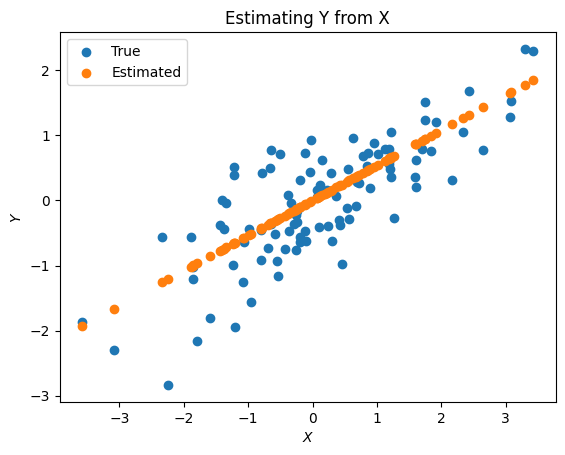
Yhat = np.matmul(A,X)

plt.scatter(X,Y,label='True')
plt.scatter(X,Yhat,label='Estimated')
plt.xlabel('$X$')
plt.ylabel('$Y$')
plt.title('Estimating Y from X')
plt.legend()
plt.show()

5.2.2.1. Estimates with a mean parameter

Suppose that instead of an estimate \( \hat y=A^T x \) , we want to include a mean vector in the estimate as \( \hat y=A^T x + \mu \) . While it is possible to derive all of the above equations for this modified model, it is easier to rewrite the model into a similar form as above with

\[\begin{split} \hat y=A^T x + \mu = \begin{bmatrix} \mu^T \\ A^T \end{bmatrix} \begin{bmatrix} 1 \\ x \end{bmatrix} := A'^T x'. \end{split}\]

That is, we can extend x by a single 1, (the observation X similarly with a row of constant 1s), and extend A to include the mean vector. With this modifications, the above Moore-Penrose pseudo-inverse can again be used to solve the modified model.

5.2.2.2. Estimates with linear equality constraints

(Advanced derivation begins)

In practical situations we often have also linear constraints, such as \( C^T A = B \) , which is equivalent with \( C^T A - B = 0. \) The modified programming task is then

\[ \min_A\, E\left[\left\|y-A^Tx\right\|^2\right]\quad\text{such that}\quad C^T A - B = 0. \]

For simplicity, let us consider only scalar estimation, where instead of vector y, as well as matrices A, B and C, respectively, we have scalar θ as well as vector a, b and *c *and the optimization problem is

\[ \min_a\, E\left[\left\|\theta-a^T x\right\|^2\right]\quad\text{such that}\quad c^T a - \beta = 0. \]

Such constraints can be included into the objective function using the method of Lagrange multipliers such that the modified objective function is

\[ \eta(a,g) = E\, \left[\left\|\theta - a^T x\right\|^2\right] - 2 \left[ \gamma \left(c^T a - \beta\right)\right]. \]

A heuristic explanation of this objective function is based on the fact the g is a free parameter. Since its value can be anything, then \( c^T a - b \) must be zero, because otherwise the output value of the objective function could be anything. That is, when optimizing with respect to a, we find the minimum of the mean square error, while simultaneously satisfying the constraint.

The objective function can further be rewritten as

\[\begin{split} \begin{split} \eta(a,g) & = E\, \left[\left(\theta - a^T x\right)\left(\theta - a^T x\right)^T\right] - 2 \gamma \left(c^T a - \beta\right) \\& = E\, \left[\theta^2 - 2\theta x^T a + a^T xx^T a\right] - 2 \gamma \left(c^T a - \beta\right) \\& = \sigma_\theta^2 + a^T R_x^T a - 2 \gamma \left(c^T a - \beta\right) \\& = \begin{bmatrix} a^T & \gamma \end{bmatrix} \begin{bmatrix} R_x & -c \\ -c^T & 0 \end{bmatrix} \begin{bmatrix} a \\ \gamma \end{bmatrix} -2 \begin{bmatrix} 0 & \beta^T \end{bmatrix} \begin{bmatrix} a \\ \gamma \end{bmatrix} + \sigma_\theta^2 \\& = \begin{bmatrix} a^T & \gamma-\beta \end{bmatrix} \begin{bmatrix} R_x & -c \\ -c^T & 0 \end{bmatrix} \begin{bmatrix} a \\ \gamma-\beta \end{bmatrix} + \text{constant} \\& := (a'-\mu)^T R' (a'-\mu) + \text{constant} . \end{split} \end{split}\]

where \( R_x = E[xx^T] \) and “constant” refers to a constant which does not depend on a or γ.

In other words, with a straightforward approach, equality constraints can in general also be merged into a quadratic form. We can therefore reduce constrained problems to unconstrained problems which can be easily solved.

Inequality constraints can be reduced to quadratic forms with similar steps as follows. Suppose we have a task \( \min f(x)\,\text{such that}\,x \geq b. \) We would then first solve the unconstrained problem \( \min f(x) \) and check whether the constraint is satisfied. If not, then the inequality constraint is “active”, that is, we must have x=b. We can then rewrite the inequality constraint as an equality constraint and solve the problem as above.

In the case that we have multiple constraints over multiple dimensions, we can keep merging them one by one until we have an entire unconstrained programming problem.

(Advanced derivation ends)

5.2.3. Some applications

• Linear prediction in modelling of the spectral envelope of speech

• Noise attenuation with Wiener filtering

5.2.4. Discussion

Linear regression is just about the simplest effective method, which you can do to model data. If that works then it’s perfect! Especially for estimating low-dimensional from high-dimensional data, linear estimates can be very useful. In any case, it is always a good approach to start modelling with the simplest possible model, which usually is a linear model. If nothing else, that gives a good baseline. The first figure on this page demonstrates a case where a linear model does do a decent job at modelling the data.

Naturally there are plenty of situations where linear models are insufficient, such as when the data

• follows non-linear relationships

• has discontinuities or when the data

• contains multiple classes with different properties.

Moreover, in many cases we are not interested in modelling the average signal, but to recreate a signal which contains all the complexity of the original signal. Say, if we want to synthesize speech, then “average speech” can sound dull. Instead, we would like to reproduce all the colorfulness and expressiveness of a natural speaker. A model of the statistical distribution of the signal can then be more appropriate, such as the Gaussian mixture model (GMM).

Another related class of models are Sub-space models, where the input signal is modeled in a lower-dimensional space such that dimensions related to background noise are cancelled and the desired speech signal is retained.