12. Self-supervised learning

Self-supervised learning (SSL) refers to a family of artificial neural network models that are used to learn useful signal representations from data without any supporting information, such as task-specific data labels. Instead of extracting manually specified signal features, such as MFCCs, SSL algorithms learn the features by taking statistical properties of the input data into acocunt. The concept of useful features refers to signal representations that can act as powerful features in a particular downstream task or a variety of tasks, for which labeled training data exists. Besides acting as a feature extractor, a pre-trained SSL model (neural network) can also be used as a model that is then trained for a downstream task. This is usually done by augmenting a trained SSL model with a small number of additional classification layers, and then training the new layers or the entire model to the target task using labeled data related to the task. This process is called model fine-tuning.

In general, SSL algorithms belong to the family of unsupervised learning algorithms and they are practically implemented as deep neural networks. The reason they are referred to as self-supervised comes from the optimization criterion used to train the models. Classical unsupervised learning operates by performing unsupervised data clustering using a heuristic algorithm (as in k-means) or by modeling the data distribution directly with a generative model (as in Gaussian mixture models, hidden-Markov models, or autoencoders). SSL algorithms, on the other hand, can be viewed as regression models (or classifiers) that try to perform regression mapping from the input data to model’s own internal representations derived from the same input data.

In case of speech data, one example of a self-supervised regression task is to predict the input speech signal over time. When a deep neural network is tasked with this prediction problem and optimized to solve it, the network has to learn higher-level properties of the data in order to solve the problem adequately. Note that the task has to be difficult enough, so that it cannot be solved by trivial means (e.g., linear interpolation from the observed values). Fig. 1 illustrates a self-supervised speech prediction task, as it is implemented in Autoregressive Predictive Coding (APC) algorithm (Chung et al., 2019). In the APC model, the task of the model is to predict spectral envelope features (e.g., log-Mel spectra or MFCCs) approximately 50 ms in the future, given access to the current and past observations of the input features.

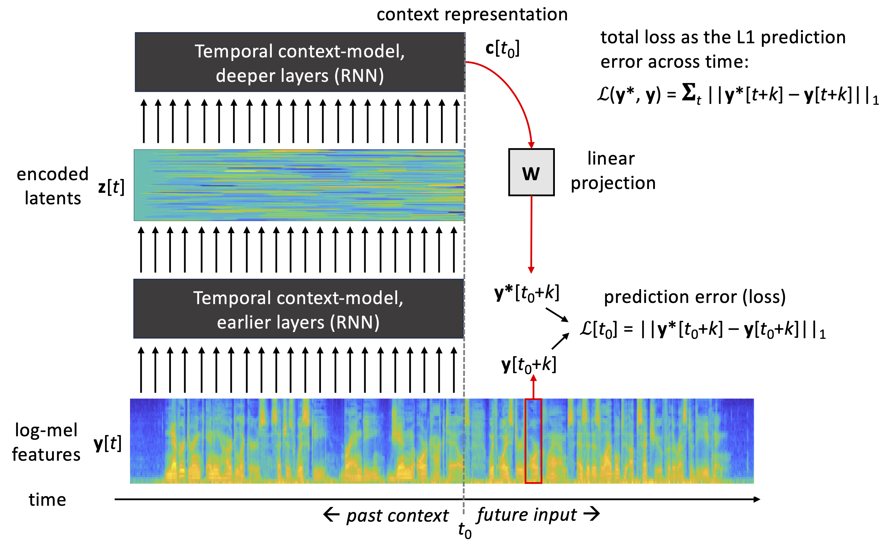
Figure 1: A schematic view of APC model for self-supervised learning. Speech signal is represented by spectral envelope features y(t), such as log-mel spectra. The APC model consists of a set of recurrent neural network layers that process the history of y[t] values up to present time, \(t \in [... ,t_0-2, t_0-1, t_0]\), producing a context representation c(\(t_0\)). The context vector is then projected linearly to produce a prediction y*[\({t_0}+k\)] of a future spectral frame y[\({t_0}+k\)] at the given prediction distance k. The mean absolute error between the predicted and true future frame is then used as the loss function and minimized during neural network training. After the training, latent vectors z(t) or context representation vectors c(t) can be used as inputs to a downstream task.

The advantage of SSL methods is that they do not require labeled data to operate, which allows their training on much larger datasets than what is typically available for a speech processing task. For instance, consider the case of deploying an automatic speech recognition (ASR) system for a new language or dialect: There may only be a few hours of representative speech data with phonemic or text transcriptions to train the system. However, there may be substantially more unlabeled speech data available in the same or similar languages. By first learning the general acoustic and statistical characteristics of speech with SSL, one can then fine-tune the system to connect the learned representations with symbolic linguistic representations of the language. This potentially results in a much more accurate ASR model than what could be achieved by applying normal supervised learning to the small labeled data directly.

In practice, SSL-based pre-training has turned out to be so powerful that a large proportion of modern speech technology systems make use of it as an integral part of the system development.

12.1. Basic archetypes of speech SSL models

SSL models for speech data can be categorized into two basic approaches: prediction and masking based models.

12.1.1. Prediction-based SSL

In the prediction-based models, the task of the neural network is to predict future evolution of the speech signal, given access to a series of past observations. This makes the models causal, as they do not access future speech observations during generation of their latent representations.

In APC (Fig. 1), the inputs and prediction targets of the neural network consist of spectral feautres (e.g. log-mel features), and the prediction distance k (in frames) is a hyperparameter defined by the user. The model itself consists of a stack of recurrent neural layers that are responsible for accumulating the history of observations… y[t-2], y[t-1], y[t] into a context vector c[t]. At every time step, the context vector is then mapped into a prediction y*[t+k] of a future feature frame at t+k using a learnable linear projection* y[t+k]=c[t]^TW.

The model is trained by minimizing the mean absolute error (MAE; aka. L1 loss) between the predicted and actual inputs across all data \(t \in [1, 2, ..., T]\):

\[ L = \sum_{t=1}^T ||{\textbf{y}}^{*}[t+k]-{\textbf{y}}[t+k]||_{1} \]

After the training, the context vectors c[t], or latent representations z[t] corresponding to activations of a chosen hidden RNN layer, can be used as features for a downstream task.

In the original APC paper, the context model was implemented as a stack of recurrent LSTM layers (1–4 layers depending on the configuration) and the prediction distance k was varied from 1 to 20 steps (10–200 ms) (Chung et al, 2019). In later works, a prediction distance of approx. 3–5 steps (30–50 ms) has been commonly adopted in many later use cases.

Contrastive Predictive Coding (CPC; van den Oord et al., 2018), illustrated in Fig. 2, is conceptually similar to APC in terms of predicting future speech using an encoder and a context model. However, instead of predicting spectral envelope of the speech at a single target distance k, CPC learns to predict its own latent vectors z[t+k] for all \(k \in {1, 2, ..., K}\) and using a separate linear projection W\(_k\) for each of the prediction distances. This means that CPC simultaneously learns the predictor and the representations to predict during training.

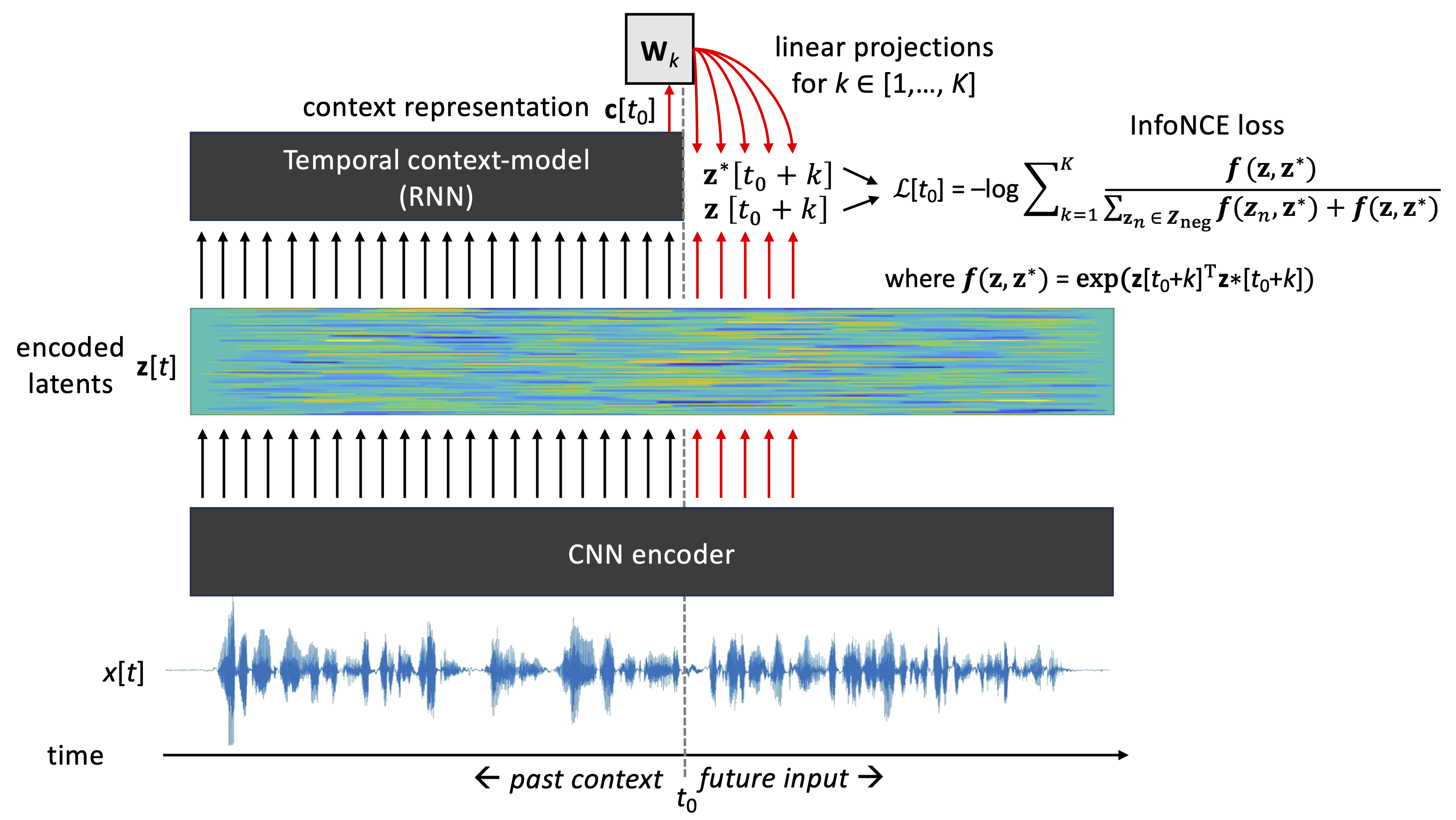
Figure 2: Illustration of the CPC algorithm (van den Oord et al., 2018). An encoder maps the input speech waveform into latent representations z[t]. An RNN-based context-model, followed by distance-specific linear mappings W\(_k\), is then used to predict future z[t+1], z[t+2], …, z[t+K] for each t in the input. At training time, a contrastive InfoNCE loss is used to optimize the predictions such that the model learns to differentiate true future latents from false futures (negative samples) drawn from the pool of latents corresponding to other time points in the input data.

When a model is allowed to invent its own prediction targets, conventional distance-based losses (e.g., L1 or L2 loss) cannot be used for model optimization due to the risk of representation collapse. During the collapse, the model learns a trivial solution for the problem, such as encoding all speech frames and their predictions with the same constant values. Although this minimizes the loss very efficiently, the resulting representations do not carry any information of the underlying signal. In CPC, representation collapse is avoided by using a so-called contrastive loss (Gutmann & Hyvärinen, 2010): instead of minimizing the distance of predicted and true future z[\(t+k\)] vectors, the model is optimized to distinguish true future observations (aka. “positive samples”) from other, usually random, observations z\(_n\)[t] produced by the same encoder (“negative samples”). Technically, this is implemented using a so-called InfoNCE loss:

By jointly optimizing the representations and their predictions, CPC learns latent representations z[t] and context representations c[t] that encode different aspects of the input speech, such as phonemic units and speaker identities, a in well-separable manner (van den Oord et al., 2018).

Note that the standard CPC uses waveforms instead of spectral features as the input, and therefore a CNN encoder is applied to map the speech into the latent space z[t] (see Fig. 2). However, the core CPC learning mechanism can also be appied to spectral feature inputs, in which case MLP encoder would be typically instead of a CNN (e.g., Chung et al., 2019; see also “Choosing between waveform and acoustic feature inputs” section below).

On the context models of prediction-based algorithms

Both APC and CPC originally use RNN-based context models (LSTMs for APC, GRUs for CPC). However, other architectures capable of temporal modeling may as well be used. These include Transformers (see, e.g., Chung & Glass, 2019, for Transformer-based APC) or WaveNet-like CNN layers that make use of dilated convolutions to efficiently capture long temporal contexts (van den Oord et al., 2016).

12.1.2. Masking-based SSL

In contrast to temporal prediction SSL models, masking based models attempt to predict parts of input data that are masked (hidden) from the network. In image domain, this would correspond to a learning problem where parts of an image are hidden from the network, and the network has to infer the contents of the hidden area (or encoded latents of it) using the surrounding visible parts of the image. In case of speech, the model typically observes several seconds of speech (e.g., an utterance), and then several temporal spans ranging from tens to hundreds of milliseconds in duration are masked from the model. Similarly to the CPC (see above), the model’s task is then to infer what kind of latent representations the model’s own encoder would generate for the masked inputs, as done by using the latent reprensetations derived from the unmasked parts of the signal.

One example of a masking based SSL is the wav2vec2.0 model (Baevski et al., 2020) illustrated in Fig. 3. In wav2vec2.0, a CNN is first used to encode speech waveform into latent z[t] similarly to CPC. However, instead of predicting in time, a subset of z[t] are masked from the subsequent Transformer layers, and the task of the final Transformer layer is to output correct predictions c[t] for the masked segments by using the surrounding context as a cue. Instead of predicting the original z[t] directly, the masked z[t] are first vector quantized (VQ) into q[t] with a learnable codebook, making the prediction targets categorical in nature. Contrastive loss is then used to optimize the network for the prediction task. An additional auxiliary loss called diversity loss is added to the total optimization loss with a weight of \(\alpha\) to ensure that the VQ process results in a hetereogenous distribution of quantization outputs.

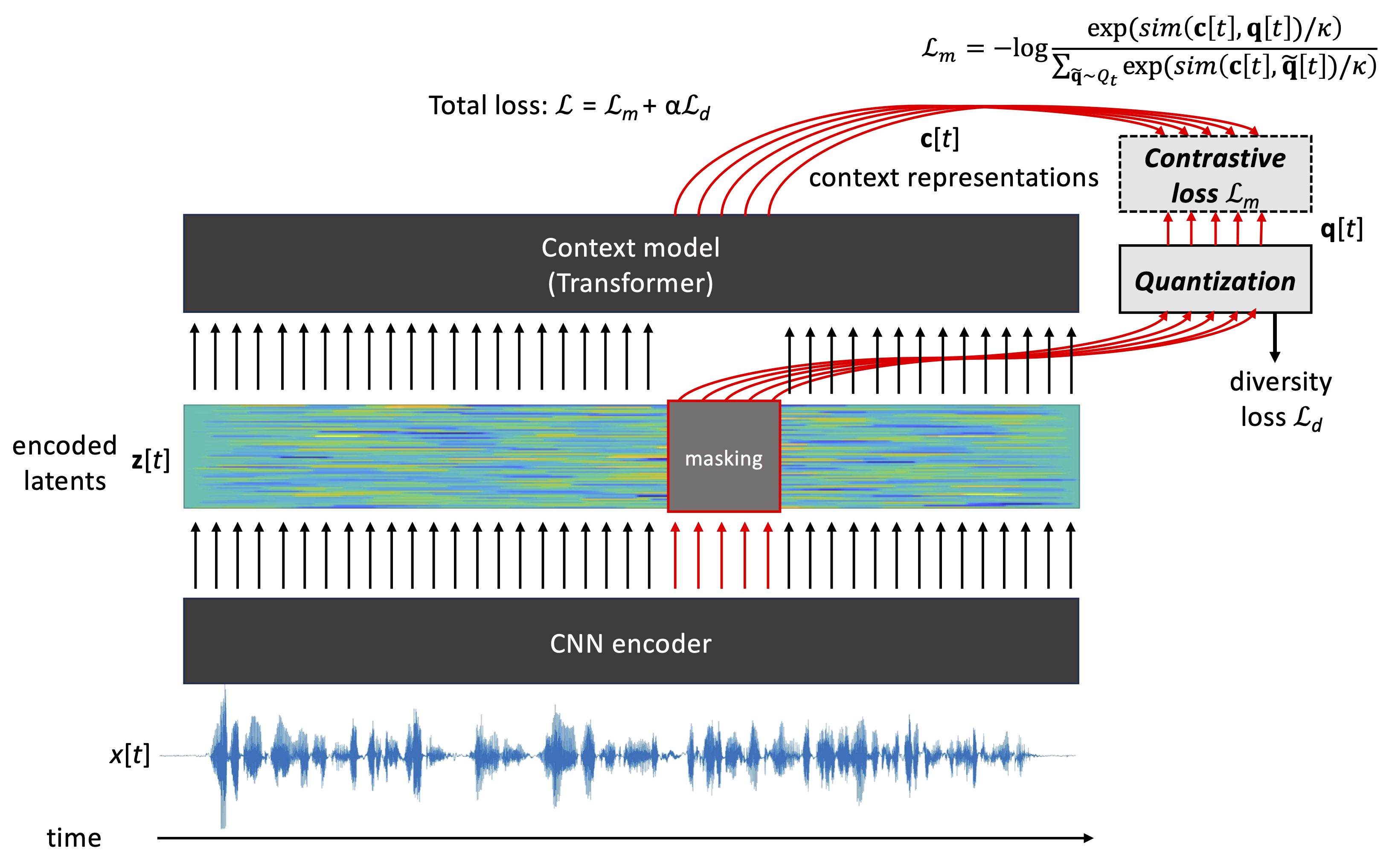
Figure 3: An illustration of wav2vec2.0 algorithm by Baevski et al. (2020). A CNN encoder produces latent short-term representations from an input waveform, one latent vector per 10 ms. A subset of these latents is then masked, and the unmasked latents are passed to a Transformer-based context model. In parallel the masked latents are vector quantized (VQ) in a separate processing branch using a learnable codebook. During training time, the model is optimized such that the Transformer correctly predicts the VQ latents of the masked input sections. A separate diversity loss is applied to the VQ to ensure that the quantization results in rich use of the quantization codebook.

Other popular masking based models include, e.g., HuBERT (Hsu et al., 2021) and data2vec (Baevski et al., 2022) algorithms. Without going into details, HuBERT learns by predicting its own Transformer layer outputs z[t] for masked sections of speech input, where the outputs are extracted from the previous training epoch of the model. During the first epoch, the targets consist of outputs of a some kind of acoustic unit discovery system, such as vector quantized spectral features. In contrast, Data2vec is a teacher-student architecture where the student network, a stack of Transformer layers, tries to predict hidden layer activations of masked input segments encoded by the teacher network. The teacher network has identical Transformer architecture to the learner, but the teacher network’s parameters are a moving average of student network parameters across several previous training epochs.

12.2. Combining SSL with downstream tasks

Once an SSL model is trained in a self-supervised manner without data labels, there are two basic ways to use the model: 1) using the model as a fixed feature extractor to provide speech features for a downstream task, or 2) using the model as a part of an end-to-end downstream task system.

In the first case, the pre-trained SSL model can simply be used as a feature extraction tool. Speech data is given as an input to the model, and then the corresponding hidden layer activations resulting from the forward pass of the model are extracted as the output features. For instance, in APC and CPC models it is common to extract encoder outputs z[t] or context vectors c[t] as short-term features for the signal at each time step t. However, activations of any hidden layer of an SSL model can be used, and the performance of the resulting features depends on the task and SSL model at hand. Usage of SSL models as frozen feature extractors is also commonly used in benchmarks used to compare performance of different SSL algorithms (e.g., Yang et al., 2021).

In the alternative use of SSL models, the pre-trained layers and weights of an SSL model are used as an encoder for a larger downstream task neural architecture. For straightforward classification and regression tasks, it is possible to directly fine-tune the SSL model to the task by simply adding an appropriate task-specific classification or regression layer after the SSL layers, and then fine-tuning some or all layers of the model using a loss function appropriate for the task. Alternatively, several new trainable layers can be appended to the SSL model before fine-tuning. The advantage of this approach is that the SSL model, including its CNN-based waveform encoder (if applicable), can benefit from the further training that optimizes the entire processing pipeline for the task at hand. The downside is that fine-tuning the entire model using a dataset of limited size can result in overfitting or catastrophic forgetting in the model. This is especially the case when there is a large number of parameters in the model. Different strategies can be utilized to mitigate such problems, such as updating only some of the deepest layers of the SSL model during the fine-tuning, reducing the learning rate of the SSL layers compared to classification layers, first training the new classification layers and then gradually proceeding to update also the earlier layers, or using special techniques such as low-rank adaptation (LoRA) that alters the behavior of the original SSL layers without directly updating their parameters (Hu et al., 2021).

12.3. Choosing between waveform and acoustic feature inputs

In the above examples, input to the APC model consisted of spectral features, such as log-mel filterbank features, which means that phase information of the signal has been discarded. Also, the less filterbank channels are used, the more the spectral envelope is averaged, which results in some loss of spectral detail, especially at high frequencies.

In contrast, CPC and wav2vec2.0 used acoustic waveforms as their default inputs. In theory, the use of the acoustic waveform provides a more general starting point for representation learning, since there is no loss of information before the SSL stage. This may provide some performance advantage over spectral features in tasks where the chosen filterbank representation is not optimal, and where there is enough data to train the waveform encoder.

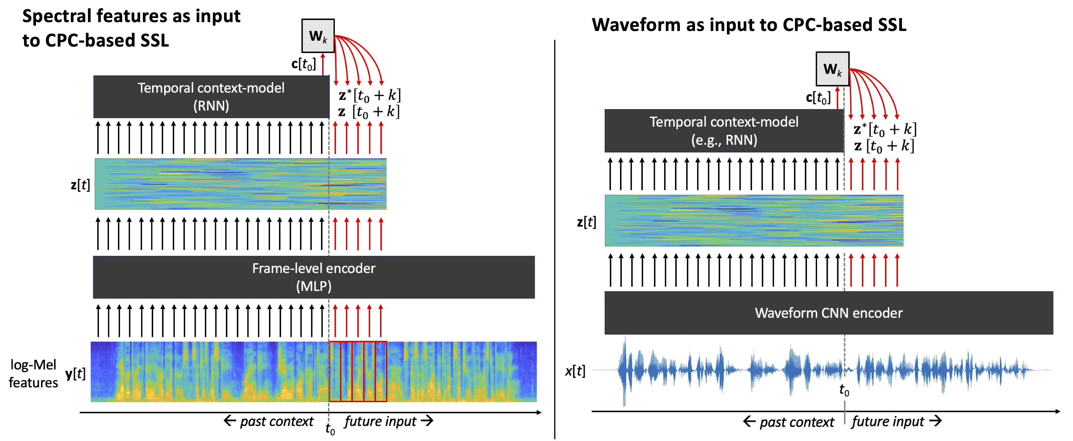
Figure 4: An illustration of CPC algorithm with two types of inputs: spectral features (left) and acoustic waveforms (right). Note the use of CNN encoder for waveforms and MLP for spectral feature frames. The core learning principles of CPC are the same in both cases, but the model naturally cannot recover information lost during the feature extraction process (such as phase information in case of log-Mel features).

In practice, nearly all of the popular SSL algorithms, such as CPC, Wav2Vec2.0, or HuBERT can use waveform or filterbank features interchangeably. The main difference is the two input types require a different type of encoder (Fig. 4):

A multilayer perceptron (MLP) can be used for spectral features, if the features are extracted at a typical frame rate (e.g., one frame every 10 ms). In this case, the goal of the encoder is to perform a (potentially complex) non-linear transformation on each of the spectral frames, mapping them to a latent representation space. In the MLP, processing of each filterbank frame is done independently of the neighboring frames, meaning that the frame rate of the encoder output is the same as in the input. Since the MLP is optimized as a part of the entire SSL model training, it learns to represent filterbank information in a manner that supports the self-supervised learning task.

A convolutional neural network (CNN) is commonly employed as the encoder when waveforms are used as inputs. In this case, the encoder serves two purposes: 1) conversion of the input signal into a form that is useful for the SSL task (as in the spectral feature case), and 2) downsampling of the signal from the original waveform sampling rate (e.g., 16 kHz) to a frame-rate compatible with the rest of the architecture and the downstream tasks, such as one frame every 10 ms. In other words, CNN can be seen as a learnable non-linear feature extractor that replaces the short-term windowing, FFT magnitude spectrum calculation, filterbank filtering, logarithmic compression, and the non-linear mapping of an MLP with a single neural module. Technically speaking, a typical CNN encoder consists of 3–5 CNN layers, where strided convolutions are employed for efficient processing of the time-domain signal, and where the effective receptive field size of the CNN corresponds to a similar 20–35 ms time-scale as in standard spectral feature calculation (e.g., van den Oord et al., 2018).

Advantages of waveform input

• All information in the signal is available to the SSL process, including signal phase and high-frequency details, allowing the neural model to determine what is useful in the signal for the task at hand.

• Maximizes performance potential of the downstream tasks, especially when further fine-tuning of the encoder can be done for the tasks.

Advantages of spectral features

• Standard features (log-mels, MFCCs) represent main spectral properties of the signal while discarding signal phase. Since phase information is not classically considered as important for most of the speech tasks, and since phase tends to vary across signal channels, the use of standard features makes the resulting SSL representations more robust against varying channel conditions (e.g., different dataset or microphone).

• Low-dimensional and well-tested speech features enable simpler models and faster learning compared to CNN having to learn to interpret time-domain samples, making them potentially more suitable for smaller data.

12.4. Benchmarking SSL models

Given the fast pace of the development of SSL methods, it may be difficult to identify the most suitable method for a particular use case. This is where standardized benchmarks for SSL performance can be of use. One such benchmark is the Speech processing Universal PERformance Benchmark (SUPERB) benchmark (Yang et al., 2021). SUPERB consists of several downstream tasks in which representations from a pre-trained SSL encoder are tested as features. These tasks include automatic speech recognition, phoneme recognition, speaker identification, speaker verification, speaker diarization, speech emotion recognition, and many more. Performance of different SSL methods in these tasks are listed on a leaderboard available at https://superbbenchmark.org/, allowing straightforward comparison of alternative methods.

12.5. References

Baevski, A., Zhou, H., Mohamed, A., & Auli, M. (2020). wav2vec 2.0: A framework for self-supervised learning of speech representations. Proc. 34th Conference on Neural Information Processing Systems (NeurIPS 2020), Vancouver, Canada.

Baevski, A., Hsu, W.-N., Xu, Q., Babu, A., Gu, J., & Auli, M. (2022). Data2vec: A General Framework for Self-supervised Learning in Speech, Vision and Language. arXiv:2202.03555

Chung, Y.-A. & Glass, J. (2019). Generative Pre-Training for Speech with Autoregressive Predictive Coding. Proc. IEEE International Conference on Acoustics, Speech and Signal Processing (ICASSP-2019), Brighton, UK, pp. 3497–3501.

Chung, Y.-A., Hsu, W.-N., Tang, H., & Glass, J. (2019). An Unsupervised Autoregressive Model for Speech Representation Learning. Proc. Interspeech-2019, Graz, Austria, pp. 146–150.

Gutmann, M. & Hyvärinen, A. (2010). Noise-contrastive estimation: A new estimation principle for unnormalized statistical models. Proc. Thirteenth International Conference on Artificial Intelligence and Statistics, pp. 297–304, 2010.

Hsu, W-N., Bolte, B., Tsai, Y-H., Lakhotia, K., & Salakhutdinov, R. (2021). HuBERT: Self-supervised speech representation learning by masked prediction of hidden units. IEEE/ACM Transactions on Audio, Speech and Language Processing, 29, pp. 3451–3460

Hu, E., Shen, Y., Wallis, P., Allen-Zhu, Z., Li, Y., Wang, S., Wang, K., & Chen, W. (2021). LoRA: Low-Rank Adaptation of Large Language Models. Proc. ICLR-2022, a virtual conference.

van den Oord, A., Dieleman, S., Zen, H., Simonyan, K., Vinyals, O., Graves, A., Kalchbrenner, N., Senior, A., & Kavukcuoglu, K. (2016). WaveNet: A Generative Model for Raw Audio. arXiv:1609.03499

van den Oord, A., Li, Y., & Vinyals, O. (2018). Representation learning with contrastive predictive coding. CoRR, abs/1807.03748.

Yang, S.-w., Chi, P.-H., Chuang, Y.-S., Lai, C.-I.J., Lakhotia, K., Lin, Y.Y., Liu, A.T., Shi, J., Chang, X., Lin, G.-T., Huang, T.-H., Tseng, W.-C., Lee, K.-t., Liu, D.-R., Huang, Z., Dong, S., Li, S.-W., Watanabe, S., Mohamed, A., Lee, H.-y. (2021). SUPERB: Speech Processing Universal PERformance Benchmark. Proc. Interspeech-2021, pp. 1194–1198.