Linear prediction¶

A random segment of a speech signal:

import numpy as np
import matplotlib.pyplot as plt
from scipy.io import wavfile
import scipy


# read from storage
filename = 'sounds/test.wav'
fs, data = wavfile.read(filename)

window_length_ms = 20
window_length = int(np.round(fs*window_length_ms/1000))

n = np.linspace(0.5,window_length-0.5,num=window_length)

windowpos = np.random.randint(int((len(data)-window_length)))

datawin = data[windowpos:(windowpos+window_length)]
datawin = datawin/np.max(np.abs(datawin)) # normalize

plt.plot(n*1000/fs,datawin)
plt.xlabel('Time (ms)')
plt.ylabel('Amplitude')
plt.title('A window of a signal')
plt.tight_layout()
plt.show()

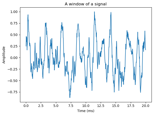
Look at the above segment of speech. What structures can you identify?

Speech is a continuous signal, which means that consecutive samples of the signal are correlated. Subsequent samples of the signal are often near each other. Moreover, the degree to which samples are near each other (the ‘nearness’) is roughly constant in a short segment.

import numpy as np
import matplotlib.pyplot as plt
from scipy.io import wavfile
import scipy


# read from storage
filename = 'sounds/test.wav'
fs, data = wavfile.read(filename)

window_length_ms = 20
window_length = int(np.round(fs*window_length_ms/1000))

n = np.linspace(0.5,window_length-0.5,num=window_length)

windowpos = np.random.randint(int((len(data)-window_length)))

datawin = data[windowpos:(windowpos+window_length)]
datawin = datawin/np.max(np.abs(datawin)) # normalize

plt.figure(figsize=(8,4))
plt.subplot(121)
plt.plot(n*1000/fs,datawin)
plt.xlabel('Time (ms)')
plt.ylabel('Amplitude')
plt.title('A window of a signal')
plt.subplot(122)
plt.plot(datawin[0:-1],datawin[1:],'.')
plt.axis('equal')
plt.title('Scatter plot of subsequent samples $x_n$ and $x_{n+1}$')
plt.xlabel('$x_{n}$')
plt.ylabel('$x_{n+1}$')
plt.tight_layout()
plt.show()

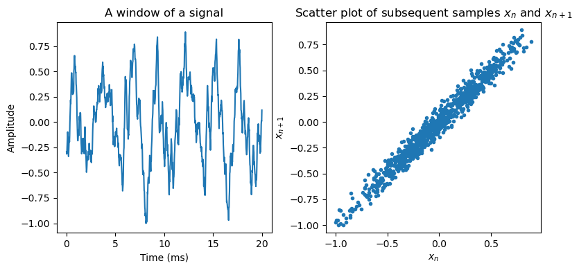
In particular, if we know a previous sample $x_{n-1}$ , we can make a prediction of the current sample, $\hat x_n = x_{n-1},$ such that $\hat x_n \approx x_n.$ By using more previous samples we have more information, which should help us make a better prediction. Specifically, we can define a predictor which uses $M$ previous samples to predict the current sample $x_{n }$ as Makhoul (1975)

\hat x_n = - \sum_{k=1}^M a_k x_{n-k}.

(1)

This is a linear predictor because it takes a linearly weighted sum of past components to predict the current one.

The error of the prediction, also known as the prediction residual is

e_n = x_n - \hat x_n = x_n + \sum_{k=1}^M a_k x_{n-k} = \sum_{k=0}^M a_k x_{n-k} = a_n * x_n

(2)

where $a_{0}=1$ . This explains why the definition of $\hat x_n$ included a minus sign; when we calculate the residual, the double negative disappears and we can collate everything into a single summation.

Vector notation¶

Using vector notation, we can make the expressions more compact

e = Xa

(3)

where

e = \begin{bmatrix}e_0\\e_1\\\vdots\\e_{N-1}\end{bmatrix},\qquad X = \begin{bmatrix} x_0 & x_{-1} & x_{-2} & \dots & x_{M} \\ x_1 & x_0 & x_{-1} & \dots & x_{M-1} \\ x_2 & x_1 & x_{0} & \dots & x_{M-2} \\ \vdots & \vdots & \vdots & & \vdots \\ x_{N-1} & x_{N-2} & x_{N-3} &\dots & x_{N-M} \end{bmatrix}, \qquad a = \begin{bmatrix}a_0\\a_1\\\vdots\\a_{M}\end{bmatrix}.

(4)

Here we calculated the residual for a length $N$ frame of the signal.

The above definition of $X$ is used in the covariance method for parameter estimation. A slight modification is to assume the input signal is windowed such that it is non-zero only for $x_0\dots x_{N-M}$ such that $x_k=0$ for $k<0$ and $k>N-M$ . It follows that $X$ becomes a convolution matrix

X = \begin{bmatrix} x_0 & 0 & \dots & 0 \\ x_1 & x_0 & \ddots & \vdots \\ x_2 & x_1 & \ddots & \vdots \\ \vdots & \vdots & \ddots & 0 \\ \vdots & \vdots & & x_0 \\ x_{N-M} & x_{N-M-1} & & \vdots \\ 0 & x_{N-M} & \ddots & \vdots\\ \vdots & \ddots & \ddots & x_{N-M-1}\\ 0 & \dots & 0 & x_{N-M} \end{bmatrix}.

(5)

The benefit of this structure is that then $X^T X$ is a Toeplitz matrix, which gives many beneficial properties in the autocovariance method below.

Parameter Estimation with the Minimum Mean-Square Error (MMSE) Approach¶

Autocovariance Method (default approach)¶

Vector $a$ holds the unknown coefficients of the predictor. To find the best possible predictor, we can minimize the minimum mean-square error (MMSE). The square error is the 2-norm of the residual, $\|e\|^2=e^T e = \sum_{k=0}^{N-1} |e_k|^2$ . The mean of that error is defined as the expectation

E\left[\|e\|^2\right] = E\left[a^T X^T X a\right] = a^T E\left[X^T X\right] a = a^T R_x a,

(6)

where $R_x = E\left[X^T X\right]$ and $E\left[\cdot\right]$ is the expectation operator. Note that, as shown in the autocorrelation section, the matrix $R_{x}$ , can be usually assumed to have a symmetric Toeplitz structure.

If we would directly minimize the mean-square error $E\left[\|e\|^2\right],$ then clearly we would obtain the trivial solution $a=0$ , which is not particularly useful. However that solution contradicts with the requirement that the first coefficient is unity, $a_{0}=1$ . In vector notation we can equivalently write

0=a_0-1=u^T a -1, \qquad\text{where}\,u=\begin{bmatrix}1\\0\\0\\\vdots\\0\end{bmatrix}.

(7)

The standard method for quadratic minimization with constraints is to use a Langrange multiplier, $\lambda$ , such that the objective function is

\eta(a,\lambda) = a^T R_x a - 2\lambda\left(a^T u - 1\right).

(8)

This function can be heuristically interpreted such that $\lambda$ is an arbitrary, free parameter. Since our objective is to minimize $a^T R_x a$ , then if $a^T u - 1$ is non-zero, then the objective function can become arbitrarily large. To allow any value for $\lambda$ , the constraint $a^T u - 1$ must therefore be zero.

The objective function is then minimized by setting its derivative with respect to $a$ to zero

0 = \frac\partial{\partial a}\eta(a,\lambda) = \frac\partial{\partial a} \left[a^T R_x a -2\lambda\left(a^T u - 1\right)\right] = 2 R_x a - 2 \lambda u.

(9)

It follows that the optimal predictor coefficients are found by solving the normal equations

R_x a = \lambda u.

(10)

Since $R_{x}$ , is symmetric and Toeplitz, the above system of equations can be efficiently solved using the Levinson-Durbin algorithm with algorithmic complexity $O(M^{2})$ . However, note that with direct solution we obtain $a':=\frac1\lambda a = R_x^{-1}u$ that is, instead of $a$ we get $a$ scaled with $\lambda$ . However, since we know that $a_{0}=1$ , we can find $a$ by $a=\lambda a' = \frac{a'}{a'_0}.$

Properties

A benefit of the autocovariance method is that the predictor is guaranteed to be stable. This means that if we use the predictor as an autoregressive model, where we iteratively predict the signal, using the previously predicted samples as input to the next prediction, then the output does not diverge. This is a convoluted (but accurate) way of saying that the predictor is usable. In the opposite case, if the filter is unstable, then with iterative predictions the output would increase exponentially for almost any input, such that with a few tens of steps the output value is larger than any convetional floating point representation. Stability is thus extremly important in practical systems which include synthesis of the signal with prediction.
Calculation of the predictor coefficients is straightforward both in the sense that it is reasonably easy to program and the computational complexity is limited.

Covariance Method¶

An alternative to the autocovariance method is to use the full signal $x_n$ without windowing, that is, without the assumption that the signal is zero outside a particular range. Then the elements of matrix $X$ at position $k,h$ can be compactly represented by $X_{k,h}=x_{k-h}$ . We can then continue to use the minimum squared error (MSE) approach to determine the coefficients $a$ , but then the covariance $C_x=X^T X$ does not have Toeplitz structure anymore. To emphasise this distinction, we talk here about the covariance $C_x=X^T X$ , whereas the autocovariance is the expectation $R_x=E[X^T X]$ .

The squared error is then $\|e\|^2 = a^T X^T X a = a^T C_x a$ . As before, we have to include the constraint $a^T u = 1$ by using the Lagrange multiplier $\lambda$ to get the objective function

\eta(a,\lambda) = a^T C_x a - 2\lambda\left(a^T u - 1\right),

(11)

whose minimum can be found be setting the partial derivative to zero as

0 = \frac{\partial}{\partial a}\eta(a,\lambda) = 2C_x a - 2\lambda u.

(12)

We do not anymore have guarantees that $C_x$ is full rank and therefore $a$ cannot be solved by inversion of $C_x$ . Instead, we have to use a pseudo-inverse signified by $^\dagger$ as

a = \lambda C_x^\dagger u.

(13)

Properties

Since this approach (arguably) does not apply windowing, it gives a more accurate representation of the system. In particular, the error is minimized for the actual system and not a biased system. Conversely, where the autocorrelation method gives a stable but biased solution, the covariance gives a more accurate but potentially unstable solution.
Since we have no guarantees for stability, this model cannot be directly used for prediction. The covariance method is therefore better suited to analysis applications.
Calculation of the pseudo-inverse typically involves solution of the singular- or eigenvalues of the matrix, which is a computationally intensive task at algorithmic complexity of ${\mathcal O}(N^3)$ .

Yule-Walker equations¶

Both the autocovariance and covariance methods involve the solution of the normal equations, of the form $Ra = \lambda u$ . However, observe that $a$ has only $M$ free parameters, but the normal equations consist of $M+1$ equations. For solution of the parameters, the scalar $\lambda$ is then just a nuisance with which we would rather do without. The normal equations can however be reduced such that $\lambda$ disappears and we have only $M$ equations left, as follows.

Observe that the normal equations can be written as

\begin{bmatrix} r_0 & r_1 & \dots & r_M \\ r_1 & r_0 & \dots & r_{M-1} \\ \vdots & \vdots & \ddots & \vdots \\ r_M & r_{M-1} & \dots & r_0 \end{bmatrix} \begin{bmatrix} 1 \\ a_1 \\ \vdots \\ a_M \end{bmatrix} = \begin{bmatrix} \lambda \\ 0 \\ \vdots \\ 0 \end{bmatrix}.

(14)

The scalar $\lambda$ is present only in the first equation, such that we can split the equations as

\begin{cases} \begin{bmatrix} r_0 & r_{1\phantom{-M}} & \dots & r_{M\phantom{-M}} \end{bmatrix} \begin{bmatrix} 1 \\ a_1 \\ \vdots \\ a_M \end{bmatrix} &= \begin{bmatrix} \lambda \end{bmatrix} \\ \begin{bmatrix} r_1 & r_0 & \dots & r_{M-1} \\ \vdots & \vdots & \ddots & \vdots \\ r_M & r_{M-1} & \dots & r_0 \end{bmatrix} \begin{bmatrix} 1 \\ a_1 \\ \vdots \\ a_M \end{bmatrix} &= \begin{bmatrix} 0 \\ \vdots \\ 0 \end{bmatrix}. \end{cases}

(15)

The first row can be discarded such that we are left with

\begin{bmatrix} 0 \\ \vdots \\ 0 \end{bmatrix} = \begin{bmatrix} r_1 & r_0 & \dots & r_{M-1} \\ \vdots & \vdots & \ddots & \vdots \\ r_M & r_{M-1} & \dots & r_0 \end{bmatrix} \begin{bmatrix} 1 \\ a_1 \\ \vdots \\ a_M \end{bmatrix} = \begin{bmatrix} r_1 \\ \vdots \\ r_M \end{bmatrix} + \begin{bmatrix} r_0 & \dots & r_{M-1} \\ \vdots & \ddots & \vdots \\ r_{M-1} & \dots & r_0 \end{bmatrix} \begin{bmatrix} a_1 \\ \vdots \\ a_M \end{bmatrix} .

(16)

Reorganizing the terms finally gives us the Yule-Walker equations as

R'a'=-r, \quad\text{where}\quad R' = \begin{bmatrix} r_0 & \dots & r_{M-1} \\ \vdots & \ddots & \vdots \\ r_{M-1} & \dots & r_0 \end{bmatrix} \quad\text{and}\quad r= \begin{bmatrix} r_1 \\ \vdots \\ r_M \end{bmatrix} \quad\text{as well as}\quad a'=\begin{bmatrix} a_1 \\ \vdots \\ a_M \end{bmatrix} .

(17)

Observe that the Yule-Walker equations are analytically equivalent with the normal equations and this rewrite is thus only for convenience. We now have $M$ unknowns in $M$ equations. However, since this equation is still best solved by the Levinson-Durbin iteration, which internally uses a version of the normal equations, and requires an extra post-processing step to support other equations, the differences in computational complexity are negligible.

Spectral properties¶

Linear prediction is usually used to predict the current sample of a time-domain signal $x_{n}$ . The usefulness of linear prediction however becomes evident by studying its Fourier spectrum (Z-transform). Specifically, since the error is a convolution of the input and the filter, $e_n = x_n*a_n$ , the corresponding Z-domain representation is

e_n=x_n*a_n \quad\Rightarrow\quad E(z) = X(z)A(z)\quad\Rightarrow\quad X(z)=\frac{E(z)}{A(z)},

(18)

where $E(z)$ , $X(z)$ , and $A(z)$ , are the Z-transforms of $e_{n}$ , $x_{n}$ and $a_{n}$ , respectively. The residual $E(z)$ is approximately white-noise, whereby the inverse $A(z)^{-1}$ , must follow the shape of $X(z)$ .

In other words, the inverse spectrum of the linear predictor $A^{-1}(z)$ thus models the macro-shape or envelope of the spectrum.

import numpy as np
import matplotlib.pyplot as plt
from scipy.io import wavfile
from scipy.linalg import solve_toeplitz
from scipy.signal import resample
import scipy


target_fs = 16000

# read from storage
filename = 'sounds/test.wav'
fs, data = wavfile.read(filename)
data = resample(data, int(len(data)*target_fs/fs))
fs = target_fs

lpc_length = int(1.25*fs/1000)
window_length_ms = 20
window_length = int(np.round(fs*window_length_ms/1000))

n = np.linspace(0.5,window_length-0.5,num=window_length)

windowpos = np.random.randint(int((len(data)-window_length)))
window_function = np.sin( np.pi*n/window_length)**2


datawin = data[windowpos:(windowpos+window_length)]
datawin = datawin/np.max(np.abs(datawin)) # normalize

# The autocorrelation of a signal is the convolution with itself r_k = x_n * x_{-n}
# which in turn is in the z-domain R(z) = |X(z)|^2. It follows that a simple way to
# calculate the autocorrelation is to take the DFT, absolute, square, and inverse-DFT.

X = scipy.fft.fft(datawin*window_function)
autocovariance = np.real(scipy.fft.ifft(np.abs(X)**2))
b = np.zeros([lpc_length+1,1])
b[0] = 1.
a = solve_toeplitz(autocovariance[0:lpc_length+1], b)
a = a/a[0]
A = scipy.fft.fft(a[:,0],n=window_length)
f = np.linspace(0,fs/1000,num=window_length)
fftlength = window_length//2

plt.figure(figsize=(12,8))
plt.subplot(221)
plt.plot(n*1000/fs,datawin)
plt.xlabel('Time (ms)')
plt.ylabel('Amplitude')
plt.title('A window of a signal')
plt.subplot(222)
plt.plot(n[0:50]*1000/fs,autocovariance[0:50])
plt.xlabel('Lag $k$ (ms)')
plt.ylabel('Autocovariance $r_k$')
plt.title('Autocovariance')
plt.subplot(223)
plt.plot(a)
plt.xlabel('Lag $k$ (ms)')
plt.ylabel('$a_k$')
plt.title(r'Predictor coefficients $a_k$ with $M=$' + str(lpc_length))
plt.subplot(224)
plt.plot(f[0:fftlength],20.*np.log10(np.abs(X[0:fftlength]/np.max(np.abs(X)))),label='Signal $X(z)$')
plt.plot(f[0:fftlength],20.*np.log10(np.abs(X[0:fftlength]*A[0:fftlength])),label='Residual $E(z)= A(z)X(z)$')
plt.plot(f[0:fftlength],3-20.*np.log10(np.abs(A[0:fftlength]/np.min(np.abs(A)))),label='Envelope $A^{-1}(z)$')
plt.xlabel('Frequency (kHz)')
plt.ylabel('Magnitude (dB)')
plt.title('Spectrum')
plt.legend()
plt.tight_layout()
plt.show()

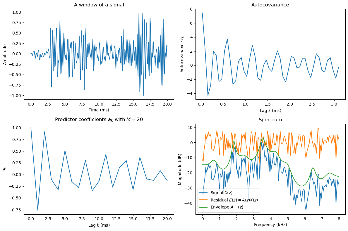
Above, we calculate the autocovariance of a random segment of a speech signal. We then calculate the corresponding predictor coefficients $a_k$ with some model order $M$ . The parameter coefficients are an abstract representation of the signal and it is generally hard to find any heuristic interpretation of the coefficients. The final panel illustrates the spectra of the signal and its envelope. We can see that the envelope follows closely the peaks of the signal. Here the envelope has been moved vertically to align approximately with the peaks, so the important observation is that the shape of the envelope follows the shape of the peaks. The absolute value (overall elevation) of the envelope is not here meaningful. Finally, we can observe that the spectrum of the residual $e_n=a_n*x_n$ is approximately flat, that is, $e_n$ is approximately white noise (statistically uncorrelated noise).

Physiological interpretation and model order¶

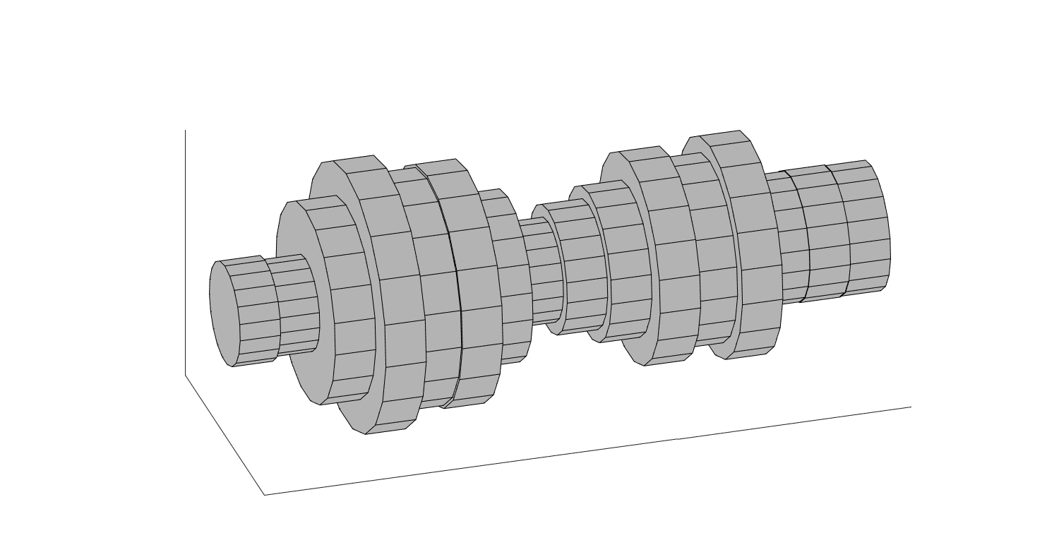
Linear prediction has a surprising connection with physical modelling of speech production. Namely, a linear predictive model is equivalent with a tube-model of the vocal tract (see figure on the right). A useful consequence is that from the acoustic properties of such a tube-model, we can derive a relationship between the physical length of the vocal tract $L$ and the number of parameters $M$ of the corresponding linear predictor as

M = \frac{2f_sL}c,

(19)

where $f_{s}$ is the sampling frequency and $c$ is the speed of sound. With an air-temperature of 35 C (approximate temperature of air flowing out from the mouth), the speed of sound is $c$ =350m/s. The mean length of vocal tracts for females and males are approximately 14.1 and 16.9 cm. We can then choose to overestimate $L$ =0.17m. At a sampling frequency of 16kHz, this gives $M\approx 17$ . The linear predictor will catch also features of the glottal oscillation and lip radiation, such that a useful approximation is $M\approx{\text{round}}\left(1.25\frac{f_s}{1000}\right)$ . For different sampling rates we then get the number of parameters $M$ as

Sampling rate $f_{s}$	Model order $M$
8 kHz	10
12.8 kHz	16
16 kHz	20

Observe however that even if a tube-model is equivalent with a linear predictor, the relationship is non-linear and highly sensitive to small errors. Moreover, when estimating linear predictive models from speech, in addition to features of the vocal tract, we will also capture features of glottal oscillation and lip-radiation It is therefore very difficult to estimate meaningful tube-model parameters from speech. A related sub-field of speech analysis is glottal inverse filtering, which attempts to estimate the glottal source from the acoustic signal. A necessary step in such inverse filtering is to estimate the acoustic effect of the vocal tract, that is, it is necessary to estimate the tube model.

A tube model of the vocal tract consisting of constant-radius tube-segments

Uses in speech coding¶

Linear prediction has been highly influential especially in early speech coders. In fact, the dominant speech coding method is code-excited linear prediction (CELP), which is based on linear prediction.

Alternative representations (advanced topic)¶

Suppose scalars $a_{m,k}$ , are the coefficients of an $M$ th order linear predictor. Coefficients of consecutive orders $M$ and $M+1$ are then related as

a_{M+1,k} = a_{M,k} + \gamma_{M+1} a_{M,M+1-k},

(20)

where the real valued scalar $\gamma_{M}\in(-1,+1)$ is the $M$ th reflection coefficient. This formulation is the basis for the Levinson-Durbin algorithm which can be used to solve the linear predictive coefficients. In a physical sense, reflection coefficients describe the amount of the acoustic wave which is reflected back in each junction of the tube-model. In other words, there is a relationship between the cross-sectional areas $S_{k}$ of each tube-segment and the reflection coefficients as

\gamma_k = \frac{S_k - S_{k+1}}{S_k + S_{k+1}}.

(21)

Furthermore, the logarithmic ratio of cross-sectional areas, also known as the log-area ratios, are defined as

A_k = \log\frac{S_k}{S_{k+1}} = \log\frac{1-\gamma_k}{1+\gamma_k}.

(22)

This form has been used in coding of linear predictive models, but is today mostly of historical interest.

Linear prediction

References

- Makhoul, J. (1975). Linear prediction: A tutorial review. Proceedings of the IEEE, 63(4), 561–580. 10.1109/PROC.1975.9792