Autocorrelation and autocovariance¶

Look at the speech signal segment below. On a large scale it is hard to discern a structure, but on a small scale, the signal seems continuous. Speech signals typically have such structure that samples near in time to each other are similar in amplitude. Such structure is often called short-term temporal structure.

More specifically, samples of the signal are correlated with the preceding and following samples. Such structures are in statistics measured by covariance and correlation, defined for zero-mean variables x and y as

\begin{split} \text{covariance: } & \sigma_{xy} = E[xy] \\ \text{correlation: } & \rho_{xy} = \frac{E[xy]}{\sqrt{E[x^2]E[y^2]}}, \end{split}

(1)

where $E[ \cdot ]$ is the expectation operator.

import numpy as np
import matplotlib.pyplot as plt
from scipy.io import wavfile
import scipy


# read from storage
filename = 'sounds/test.wav'
fs, data = wavfile.read(filename)

window_length_ms = 20
window_length = int(np.round(fs*window_length_ms/1000))

n = np.linspace(0.5,window_length-0.5,num=window_length)

#windowpos = np.random.randint(int((len(data)-window_length)))
windowpos = 92274

datawin = data[windowpos:(windowpos+window_length)]
datawin = datawin/np.max(np.abs(datawin)) # normalize

plt.plot(n*1000/fs,datawin)
plt.xlabel('Time (ms)')
plt.ylabel('Amplitude')
plt.title('A window of a signal')
plt.tight_layout()
plt.show()

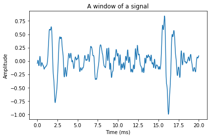
For a speech signal $x_{n}$ , where $n$ is the time-index, we would like to measure the correlation between two time-indices $x_{n}$ and $x_{h}$ . Since the structure which we are interested in appears when $n$ and $h$ are near each other, it is better to measure the correlation between $x_{n}$ and $x_{n-k}$ . The scalar $k$ is known as the lag. Furthermore, we can assume that the correlation is uniform over all $n$ within the segment. The self-correlation and -covariances, known as the autocorrelation and autocovariance are defined as

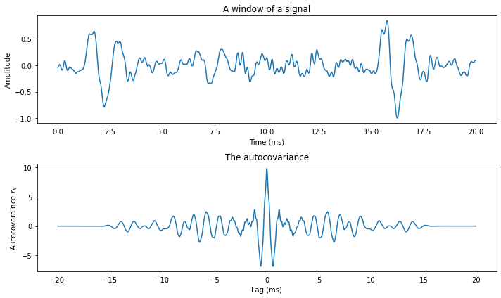
\begin{split} \text{autocovariance: } & r_{k} = E_n[x_nx_{n-k}] \\ \text{autocorrelation: } & c_{k} = \frac{E_n[x_nx_{n-k}]}{E_n[x_n^2]} = \frac{r_k}{r_0}. \end{split}

(2)

The figure below illustrates the autocovariance of the above speech signal. We can immediately see that the short-time correlations are preserved - on a small scale, the autocovariance looks similar to the original speech signal. The oscillating structure is also accurately preserved.

Because we assume that the signal is stationary, and as a consequence of the above formulations, we can readily see that autocovariances and -correlations are symmetric

r_k = E_n[x_nx_{n-k}] = E_n[x_{n+k}x_{n+k-k}] = E_n[x_{n+k}x_{n}] = r_{-k}.

(3)

This symmetry is clearly visible in the figure below, where the curve is mirrored around lag 0.

import numpy as np
import matplotlib.pyplot as plt
from scipy.io import wavfile
import scipy
import scipy.fft


# read from storage
filename = 'sounds/test.wav'
fs, data = wavfile.read(filename)

window_length_ms = 20
window_length = int(np.round(fs*window_length_ms/1000))

n = np.linspace(0.5,window_length-0.5,num=window_length)
n2 = np.linspace(1-window_length,window_length-1,num=window_length*2)

# windowing function
windowing_fn = np.sin(np.pi*n/window_length)**2 # sine-window


#windowpos = np.random.randint(int((len(data)-window_length)))
windowpos = 92274

datawin = data[windowpos:(windowpos+window_length)]
datawin = datawin/np.max(np.abs(datawin)) # normalize

spectrum = scipy.fft.rfft(datawin*windowing_fn,n=2*window_length)
autocovariance = scipy.fft.irfft(np.abs(spectrum**2))
autocovariance = np.concatenate((autocovariance[window_length:],autocovariance[0:window_length]))

plt.figure(figsize=[10,6])
plt.subplot(211)
plt.plot(n*1000/fs,datawin)
plt.xlabel('Time (ms)')
plt.ylabel('Amplitude')
plt.title('A window of a signal')
plt.subplot(212)
plt.plot(n2*1000/fs,autocovariance)
plt.xlabel('Lag (ms)')
plt.ylabel('Autocovaraince $r_k$')
plt.title('The autocovariance')
plt.tight_layout()
plt.show()

The above formulas use the expectation operator $E[\cdot ]$ to define the autocovariance and -correlation. It is an abstract tool, which needs to be replaced by a proper estimator for practical implementations. Specifically, to estimate the autocovariance from a segment of length $N$ , we use

r_k \approx \frac1{N-1} \sum_{k=1}^{N-1} x_n x_{n-k}.

(4)

Observe that the speech signal $x_{n}$ has to be windowed before using the above formula.

We can also make an on-line estimate (a.k.a. leaky integrator) of the autocovariance for sample position $n$ with lag $k$ as

\hat r_k(n) := \alpha x_n x_{n-k} + (1-\alpha) \hat r_k(n-1),

(5)

where $\alpha\in[0,1]$ is a small positive constant which determines how rapidly the estimate converges.

It is often easier to work with vector notation instead of scalars, whereby we need the corresponding definitions for autocovariances. Suppose

x = \begin{bmatrix}x_0\\x_1\\\vdots\\x_{N-1}\end{bmatrix}.

(6)

We can then define the autocovariance matrix as

R_x := E[x x^T] = \begin{bmatrix}E[x_0^2] & E[x_0x_1] & \dots & E[x_0x_{N-1}]\\E[x_1x_0] & E[x_1^2] & \dots & E[x_1x_{N-1}]\\\vdots&\vdots&\ddots&\vdots\\E[x_{N-1}x_0] & E[x_{N-1}x_1] & \dots & E[x_{N-1}^2]\end{bmatrix} = \begin{bmatrix}r_0 & r_1 & \dots & r_{N-1}\\ r_1 & r_0 & \dots & r_{N-2}\\\vdots&\vdots&\ddots&\vdots\\r_{N-1} & r_{N-1} & \dots & r_0\end{bmatrix}.

(7)

Clearly $R_{x}$ is thus a symmetric Toeplitz matrix. Moreover, since it is a product of $x$ with itself, $R_{x}$ is also positive (semi-)definite.