Introduction
The fundamental frequency of a speech signal, often denoted by F0 or , refers to the approximate frequency of the (quasi-)periodic structure of voiced speech signals. The oscillation originates from the vocal folds, which oscillate in the airflow when appropriately tensed. The fundamental frequency is defined as the average number of oscillations per second and expressed in Hertz. Since the oscillation originates from an organic structure, it is not exactly periodic but contains significant fluctuations. In particular, amount of variation in period length and amplitude are known respectively as jitter and shimmer. Moreover, the F0 is typically not stationary, but changes constantly within a sentence. In fact, the F0 can be used for expressive purposes to signify, for example, emphasis and questions.
Typically fundamental frequencies lie roughly in the range 80 to 450 Hz, where males have lower voices than females and children. The F0 of an individual speaker depends primarily on the length of the vocal folds, which is in turn correlated with overall body size. Cultural and stylistic aspects of speech naturally have also a large impact.
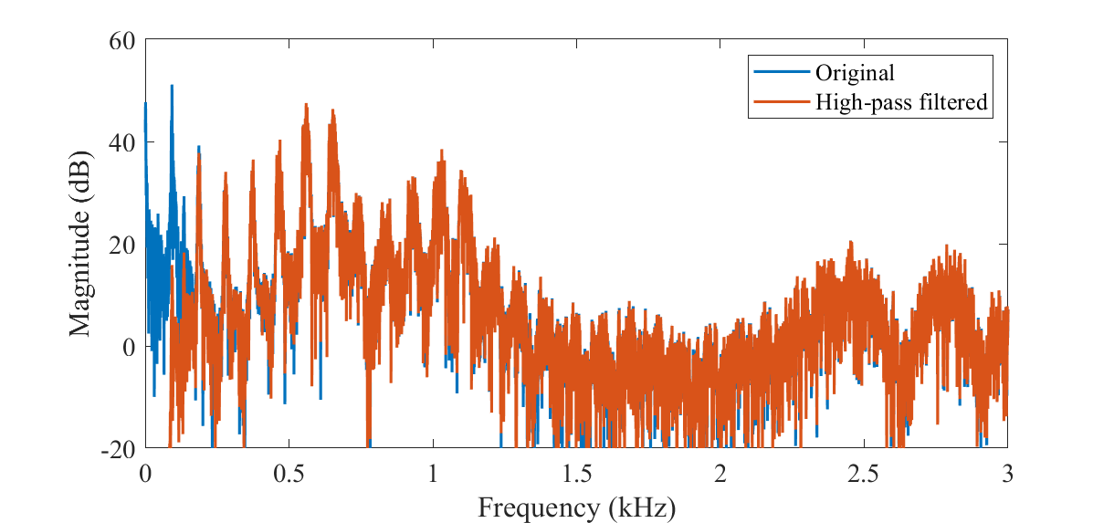
The fundamental frequency is closely related to pitch, which is defined as our perception of fundamental frequency. That is, the F0 describes the actual physical phenomenon, whereas pitch describes how our ears and brains interpret the signal, in terms of periodicity. For example, a voice signal could have an F0 of 100 Hz. If we then apply a high-pass filter to remove all signal components below 450 Hz, then that would remove the actual fundamental frequency. The lowest remaining periodic component would be 500 Hz, which correspond to the fifth harmonic of the original F0. However, a human listener would then typically still perceive a pitch of 100 Hz, even if it does not exist anymore. The brain somehow reconstructs the fundamental from the upper harmonics. This well-known phenomenon is however still not completely understood.
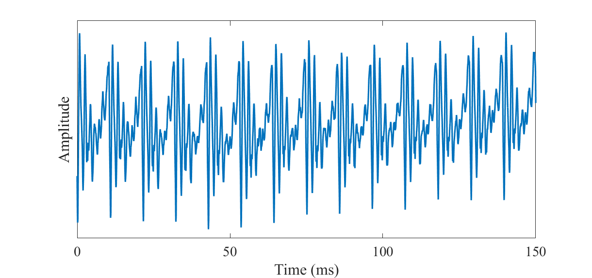
A speech signal with a fundamental frequency of approximately F0=93Hz.
The spectrum of a speech signal with a fundamental frequency of approximately F0=93Hz (original) and a high-pass filtered version of it such that the fundamental frequency has been removed (high-pass filtered).
A speech signal with a fundamental frequency of approximately F0=93Hz

Source
import IPython.display as ipd
ipd.Audio('attachments/175515683.wav')A high-pass filtered version of it such that the fundamental frequency has been removed
Source
import IPython.display as ipd
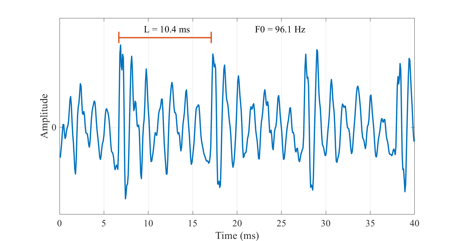
ipd.Audio('attachments/175515684.wav')If is the fundamental frequency, then the length of a single period in seconds is
The speech waveform thus repeats itself after every seconds.
A simple way of modelling the fundamental frequency is to repeat the signal after a delay of seconds. If a signal is sampled with a sampling rate of , then the signal repeats after a delay of samples where
A signal then approximately repeats itself such that
In the Z-domain this can be modelled by an IIR-filter as
where the scalar scales with the accuracy of the period. The Z-transform of the signal can then be written as where is the Z-transform of a single period.
Segment of a speech signal, with the period length , and fundamental
frequency .
Spectrum of speech signal with the fundamental frequency and harmonics , as well as the formants F1, F2, F3... Notice how the harmonics form a regular comb-structure.
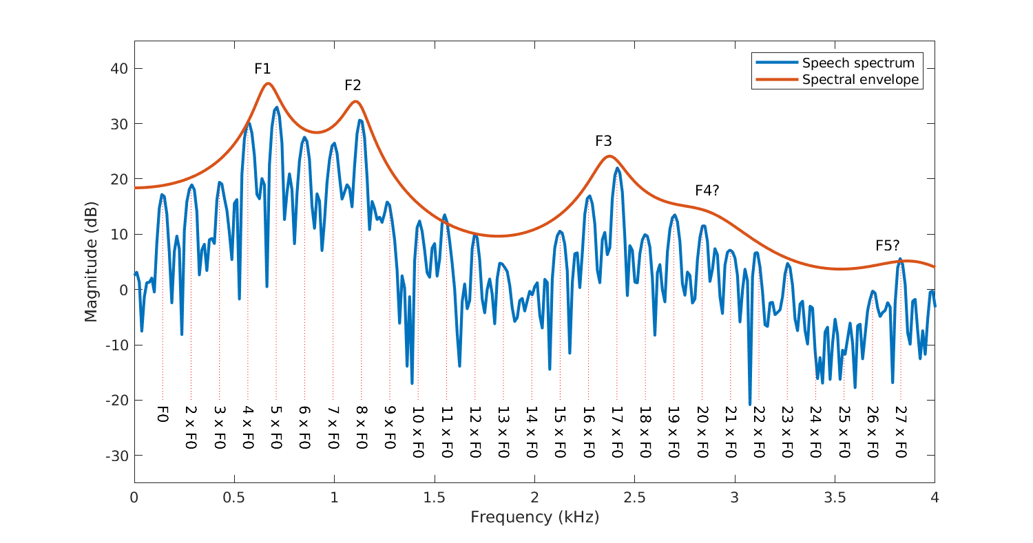
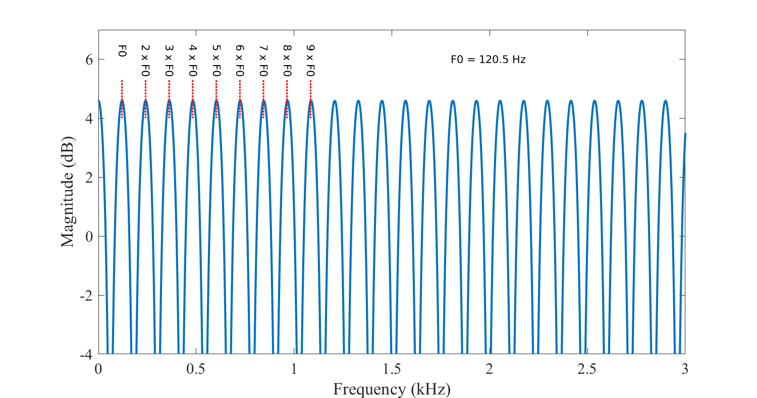
The magnitude spectrum of , has then a periodic comb-structure. That is, the magnitude spectrum has peaks at , for integer . For a discussion about the fundamental frequency in the cepstral domain, see Cepstrum and MFCC.
Spectrum of fundamental frequency model , showing the characteristic comb-structure with harmonic peaks appearing at integer multiples of .
Fundamental frequency estimation
The fundamental frequency (F0) is central in describing speech signals whereby we need methods for estimating the from speech signals. In speech analysis applications, it can be informative to study the absolute value of the fundamental frequency as such, but more commonly, extraction of the is usually a pre-processing step. For example, in recognition tasks, is often used as a feature for machine learning methods. A voice activity detector could, for instance, set a lower and higher threshold on the , such that sounds with an outside the valid range would be classified as non-speech.
The fundamental frequency is visible in multiple different domains:
In an acoustic time signal, the is visible as a repetition after every samples.
In the autocovariance or -correlation, the is visible as a peak at lag as well as its integer multiples .
In the magnitude, power or log-magnitude spectrum, the is visible as a peak at the frequency , as well as its integer multiples, where is the sampling frequency.
In the cepstrum, the is visible as a peak at quefrency as well as its integer multiples .
Consequently, we can use any of these domains to estimate the fundamental frequency . A typical approach applicable in all domains except the time domain is peak-picking. The fundamental frequency corresponds to a peak in each domain, such that we can determine the by finding the highest peak. For better robustness to spurious peaks and computational efficiency, we naturally limit our search to the range of valid ’s, such as
The harmonic structure, however, poses a problem for peak-picking. Peaks appear at integer multiples of either or lag T, such that sometimes, by coincidence or due to estimation errors, the harmonic peaks can be higher than the primary peak. Such estimation errors are known as octave errors because the error in corresponds to the musical interval of an octave. A typical post-processing step is, therefore, to check for octave jumps. We can check whether or correspond to a sensible . Alternatively, we can check whether the previous analysis frame had an , an octave, or two octaves off. Depending on the application, we can then fix errors or label problematic zones for later use.
Another problem with peak picking is that peak locations might not align with the samples. For example, in the autocorrelation domain, the actual length of the period could be 100.3 samples. However, the peak in the autocorrelation would then appear at lag 100. One approach would then be to use quadratic interpolation between samples near a peak and use the location of the maximum of the interpolated peak to estimate the peak location. Interpolation makes the estimate less sensitive to noise. For example, background noise could peak at lag 102, so the desired maximum of 100 is lower than the peak at 102. By using data from more samples, as in the interpolation approach, we can, therefore, reduce the likelihood that a single corrupted data point would cause an error.
An alternative approach to peak-picking is to use all distinctive peaks to estimate the jointly. That is, if you find peaks at frequencies , which approximately correspond to harmonic peaks , then you can approximate Another alternative is to calculate the distance between consecutive peaks and estimate We can also combine these methods as we like.
A further potential improvement is to compare subsequent frames. The pitch in speech is fairly continuous over time, and subsequent frames should, therefore, have similar F0s. This can be used to reduce the danger of octave jumps.
In many other applications, we use discrete Fourier transform (DFT) or cosine transforms (DCT) to resolve frequency components. It would, therefore, be tempting to apply the same approach here. In such a domain, we would also already have a joint estimate which does not rely on single data points. However, note that the spectrum is already the DFT of the time signal, and the cepstrum is the DCT or DFT of the log-spectrum. Additional transforms, therefore, usually do not resolve the ambiguity between harmonics.
A classic algorithm for fundamental frequency estimation is YIN De Cheveigné & Kawahara (2002), which has been later improved with a probabilistic version pYIN Mauch & Dixon (2014). YIN is based on peak picking in the autocorrelation domain while emphasizing continuity over time.
Examples
Source
# Initialization
import matplotlib.pyplot as plt
from scipy.io import wavfile
import scipy
import scipy.fft
import numpy as np
import IPython

filename = 'sounds/f0sample.wav'

#plt.rcParams.update({
#    "text.usetex": True,
#    "font.family": "Helvetica"
#})

# read from storage
fs, data = wavfile.read(filename)
data = data[:,0]
time = np.arange(len(data))/fs

IPython.display.display(IPython.display.Audio(data,rate=fs))
plt.figure(figsize=(6,3))
plt.plot(time,data)
plt.xlabel('Time (s)')
plt.ylabel('Amplitude')
plt.yticks([])
plt.show()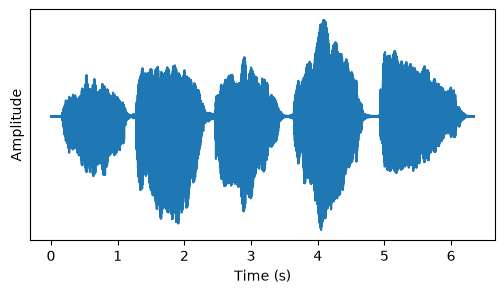
Excerpts of each tone (columns) with a square (upper row) and a Hann window (lower row).
Source
window_length_ms = 30

window_length = int(window_length_ms*fs/1000)
window_time = np.arange(window_length)
windowing_function = np.sin(np.pi*np.arange(0.5,window_length,1)/window_length)**2


time_sec_list = [0.7, 1.7, 3, 4.1, 5.4]
plt.figure(figsize=(8,4))

for k in range(5):
    time_ix = int(time_sec_list[k]*fs) + window_time
    plt.subplot(251+k)
    plt.plot(time_ix/fs, data[time_ix])
    if k==0: plt.ylabel('Amplitude')
    plt.yticks([])
    plt.subplot(2,5,6+k)
    plt.plot(time_ix/fs, data[time_ix]*windowing_function)
    plt.xlabel('Time (s)')
    if k==0: plt.ylabel('Amplitude')
    plt.yticks([])

plt.tight_layout()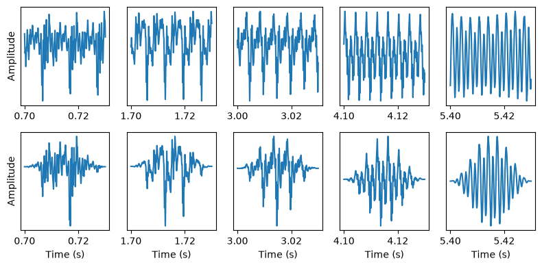
The (loosly) periodic structure is visible for each tone as a repeated waveform. Left to right, the pitch increases and the period length becomes shorter such that more periods fit the 30ms analysis window. We also note that for the lowest tone, the periods are nicely visible with the square window (upper row), but less so with the Hann window.
To estimate the fundamental frequency, recall that for a zero-mean signal with a period length , we should have or equivalently, zero expectation For a sample segment of length , the expectation has
Here is a vector containing the samples of to .
To find the fundamental frequency, we can then find that where the above norm is closest to zero.
where constants that do not depend on were omitted, and the minimum was replaced by the maximum by changing the sign. We thus obtained the maximization of the correlation between the signal and its delayed version. Note that this makes this approach equivalent with estimating the maximum of the autocorrelation function.
f0_range_Hz = np.array([80, 450])
f0_range = np.round(fs/np.flipud(f0_range_Hz)).astype(int)

print(f"Frequency range {f0_range_Hz[0]} to {f0_range_Hz[1]} Hz. "
      f"Lag range {(1000/f0_range_Hz[1]):2.2f} to {(1000/f0_range_Hz[0]):2.2f} ms or\n{f0_range[0]} to {f0_range[1]} samples with the sampling rate {fs/1000} kHz.")

correlation = np.zeros([5,window_length-1])

for k in range(5):
    time_ix = int(time_sec_list[k]*fs) + window_time
    xwin = data[time_ix]*windowing_function
    for L in range(window_length-1):
        x_k = xwin[:window_length-L]
        x_kL = xwin[L:window_length]
        correlation[k,L] = np.sum(x_k*x_kL)/(window_length-L)

max_lag = np.argmax(correlation[:,f0_range[0]:f0_range[1]],axis=1)+f0_range[0]
Frequency range 80 to 450 Hz. Lag range 2.22 to 12.50 ms or
98 to 551 samples with the sampling rate 44.1 kHz.
To make comparisons between the estimators in this chapter concrete, we score each one against a reference pitch using the mean absolute error (MAE), expressed in cents -- a logarithmic, perceptually motivated unit of pitch distance in which 100 cents make a semitone and 1200 cents make an octave:
where is the estimated and the reference pitch of frame . Cents make errors comparable across octaves -- an octave error is always 1200 cents, whether it happens at 100 Hz or at 400 Hz -- which a plain difference in Hz would not. We use pYIN’s own estimate as the reference throughout this chapter, since it is consistently the most accurate of the methods discussed here, though, as the closing Discussion of this chapter points out, it remains an estimate rather than a true ground truth. To keep the many figures below comparable, we also fix one colour per estimator for the remainder of the chapter.
Source
import librosa

# One colour per estimator, reused in every figure for the rest of this
# chapter.
method_colors = {
    'Correlation': 'tab:blue',
    'Spectrum':    'tab:orange',
    'Cepstrum':    'tab:green',
    'pYIN':        'tab:red',
    'PENN':        'tab:purple',
}

def mae_cents(estimate, reference, mask=None):
    """Mean absolute error between two pitch estimates, in cents."""
    estimate = np.asarray(estimate)
    reference = np.asarray(reference)
    if mask is not None:
        estimate = estimate[mask]
        reference = reference[mask]
    return np.mean(np.abs(1200*np.log2(estimate/reference)))

# A pYIN estimate of each tone's pitch, used below as the reference against
# which we score the Correlation/Spectrum/Cepstrum estimates.
f0pyin_tones, _, _ = librosa.pyin(data.astype(float), sr=fs,
                                   fmin=f0_range_Hz[0], fmax=f0_range_Hz[1],
                                   frame_length=window_length, hop_length=window_length//4)
pyin_tone_times = librosa.times_like(f0pyin_tones, sr=fs, hop_length=window_length//4)
tone_reference = np.array(
    [f0pyin_tones[np.argmin(np.abs(pyin_tone_times - t))] for t in time_sec_list])
Source
plt.figure(figsize=(8,5))
for k in range(5):
    plt.subplot(2,5,1+k)
    plt.plot(1000*np.arange(window_length-1)/fs, correlation[k,:], color=method_colors['Correlation'])
    plt.xlabel('Lag $L$ (ms)')
    if k==0: plt.ylabel('Correlation')
    plt.yticks([])
    plt.xticks([0, 15,30])

    plt.subplot(2,5,6+k)
    plt.plot(1000*np.arange(window_length-1)/fs, correlation[k,:], color=method_colors['Correlation'])
    plt.plot(1000*np.array([f0_range[0], f0_range[0], f0_range[0], f0_range[1], f0_range[1], f0_range[1]])/fs,
             correlation[k,0]*np.array([1.15, 1.05, 1.1, 1.1, 1.05, 1.15]),color='red')

    plt.plot(1000*max_lag[k]/fs, correlation[k,max_lag[k]], 'rx')
    plt.title(f"Peak at lag {max_lag[k]}, \nor {fs/max_lag[k]:2.1f} Hz")
    plt.xlabel('Lag $L$ (ms)')
    if k==0: plt.ylabel('Correlation')
    plt.yticks([])
    plt.xticks([0, 15])
    plt.xlim([-1, 16])


plt.tight_layout()
plt.show()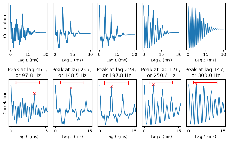
Source
print(f"Correlation: {mae_cents(fs/max_lag, tone_reference):.0f} cents MAE vs pYIN")
Correlation: 7 cents MAE vs pYIN
The upper row shows the whole correlation, while the lower row zooms near the valid range of lags (indicated by the red lines). Red crosses show the maximum peak.
With this easy sound example, the maxima are easy to discern. However, with both the lowest (leftmost) and highest (rightmost) pitches, other peaks are very close in magnitude to the true pitch. As this was an easy signal, it is thus not difficult to imagine more challenging sounds where peak picking would land at the incorrect peak.
We can repeat the experiment using the power spectrum (squared absolute spectrum).
fft_length = window_length
spectrum_length = (fft_length//2)+1
f0_range_fft_indices = np.round(f0_range_Hz*fft_length/fs).astype(int)

power_spectrum = np.zeros([5,spectrum_length])
for k in range(5):
    time_ix = int(time_sec_list[k]*fs) + window_time
    xwin = data[time_ix]*windowing_function
    power_spectrum[k,:] = np.abs(scipy.fft.rfft(xwin,n=fft_length))**2

max_frequency_index = np.argmax(
    power_spectrum[:,f0_range_fft_indices[0]:f0_range_fft_indices[1]],
    axis=1) +f0_range_fft_indices[0]
max_frequency = max_frequency_index*fs/fft_length
Source
fft_ix = np.linspace(0,fs/2,spectrum_length)
plot_range_Hz = np.arange(0, 1200)
plot_range = np.round(plot_range_Hz*fft_length/fs).astype(int)

plt.figure(figsize=(8,5))
for k in range(5):
    plt.subplot(2,5,1+k)
    plt.plot(fft_ix/1000, 10*np.log10(power_spectrum[k,:]), color=method_colors['Spectrum'])
    plt.xlabel('Frequency (kHz)')
    if k==0: plt.ylabel('Power (dB)')
    plt.yticks([])

    plt.subplot(2,5,6+k)
    plt.plot(fft_ix[plot_range],
             10*np.log10(power_spectrum[k,plot_range]), color=method_colors['Spectrum'])
    plt.plot(np.array([f0_range_Hz[0],
                            f0_range_Hz[0],
                            f0_range_Hz[0],
                            f0_range_Hz[1],
                            f0_range_Hz[1],
                            f0_range_Hz[1]]),
             10*np.log10(np.max(power_spectrum[k,:]))*np.array([1.15, 1.05, 1.1, 1.1, 1.05, 1.15]),color='red')

    plt.plot(max_frequency[k],
             10*np.log10(power_spectrum[k,max_frequency_index[k]]),
             'rx')
    plt.title(f"Peak at index {max_frequency_index[k]}, \nor {max_frequency[k]:2.1f} Hz")
    plt.xlabel('Frequency (Hz)')
    if k==0: plt.ylabel('Power (dB)')
    plt.yticks([])
    plt.xlim([-1, 1000])


plt.tight_layout()
plt.show()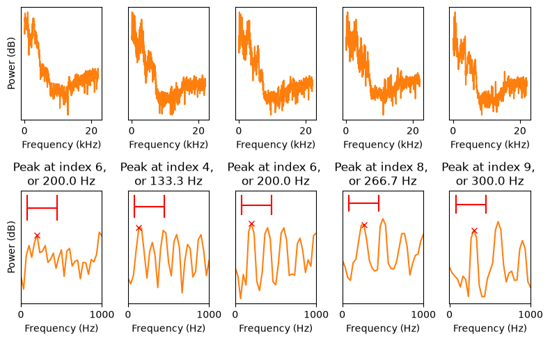
Source
print(f"Spectrum (narrowband FFT): {mae_cents(max_frequency, tone_reference):.0f} cents MAE vs pYIN")
Spectrum (narrowband FFT): 315 cents MAE vs pYIN
Observe that the y-axis is now expressed in decibels. The upper row has the complete spectrum of each tone, while the lower row zooms in on the frequency range where the fundamental is visible.
We immediately observe that for the lowest (leftmost) tone, the pitch is incorrectly estimated as it picks up the second peak of the harmonic structure. In fact, for the two highest pitches, the second harmonic peak is higher than the first, but it is not incorrectly picked up only because it is outside the defined frequency analysis range. Furthermore, the accuracy of estimated frequencies is low because that the density of frequencies is not sufficient. The accuracy can however be improved by oversampling the spectrum, that is, by extending the analysis window by zeros before the Fourier transform.
In other words, let us extend the vector with zeros to a length equal to the sampling rate (44100).
Source
fft_length = fs
spectrum_length = (fft_length//2)+1
f0_range_fft_indices = np.round(f0_range_Hz*fft_length/fs).astype(int)

power_spectrum = np.zeros([5,spectrum_length])
for k in range(5):
    time_ix = int(time_sec_list[k]*fs) + window_time
    xwin = data[time_ix]*windowing_function
    power_spectrum[k,:] = np.abs(scipy.fft.rfft(xwin,n=fft_length))**2

max_frequency_index = np.argmax(
    power_spectrum[:,f0_range_fft_indices[0]:f0_range_fft_indices[1]],
    axis=1) +f0_range_fft_indices[0]
max_frequency = max_frequency_index*fs/fft_length
Source
fft_ix = np.linspace(0,fs/2,spectrum_length)
plot_range_Hz = np.arange(0, 1200)
plot_range = np.round(plot_range_Hz*fft_length/fs).astype(int)

plt.figure(figsize=(8,3))
for k in range(5):
    plt.subplot(2,5,1+k)
    plt.plot(fft_ix[plot_range],
             10*np.log10(power_spectrum[k,plot_range]), color=method_colors['Spectrum'])
    plt.plot(np.array([f0_range_Hz[0],
                            f0_range_Hz[0],
                            f0_range_Hz[0],
                            f0_range_Hz[1],
                            f0_range_Hz[1],
                            f0_range_Hz[1]]),
             10*np.log10(np.max(power_spectrum[k,:]))*np.array([1.15, 1.05, 1.1, 1.1, 1.05, 1.15]),color='red')

    plt.plot(max_frequency[k],
             10*np.log10(power_spectrum[k,max_frequency_index[k]]),
             'rx')
    plt.title(f"Peak at index {max_frequency_index[k]}, \nor {max_frequency[k]:2.1f} Hz")
    plt.xlabel('Frequency (Hz)')
    if k==0: plt.ylabel('Power (dB)')
    plt.yticks([])
    plt.xlim([-1, 1000])


plt.tight_layout()
plt.show()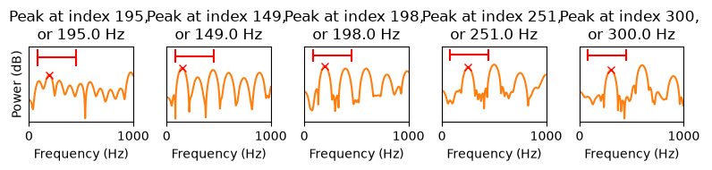
Source
print(f"Spectrum (oversampled FFT): {mae_cents(max_frequency, tone_reference):.0f} cents MAE vs pYIN")
Spectrum (oversampled FFT): 244 cents MAE vs pYIN
It is now much easier to determine the exact location of each peak and thus the frequency estimates are also more accurate. However, this did not solve the octave jump in the lowest (leftmost) tone, where the second harmonic is still larger than the first, true peak.
The third main feature often used for F0 estimation is the cepstrum.
Source
fft_length = window_length
spectrum_length = (fft_length//2)+1
f0_range_fft_indices = np.round(f0_range_Hz*fft_length/fs).astype(int)

power_spectrum = np.zeros([5,spectrum_length])
for k in range(5):
    time_ix = int(time_sec_list[k]*fs) + window_time
    xwin = data[time_ix]*windowing_function
    power_spectrum[k,:] = np.abs(scipy.fft.rfft(xwin,n=fft_length))**2
cepstrum = scipy.fft.irfft(10*np.log10(power_spectrum),axis=1)
max_cepstral_peak = np.argmax(cepstrum[:,f0_range[0]:f0_range[1]],axis=1)+f0_range[0]Source
plt.figure(figsize=(8,3))
for k in range(5):
    plt.subplot(1,5,1+k)
    plt.plot(1000*np.arange(window_length-1)/fs, cepstrum[k,:], color=method_colors['Cepstrum'])
    plt.plot(1000*np.array([f0_range[0], f0_range[0], f0_range[0], f0_range[1], f0_range[1], f0_range[1]])/fs,
             cepstrum[k,max_cepstral_peak[k]]*np.array([1.55, 1.35, 1.4, 1.4, 1.35, 1.55]),color='red')

    plt.plot(1000*max_cepstral_peak[k]/fs, cepstrum[k,max_cepstral_peak[k]], 'rx')
    plt.title(f"Peak at lag {max_cepstral_peak[k]}, \nor {fs/max_cepstral_peak[k]:2.1f} Hz")
    plt.xlabel('Quefrency $L$ (ms)')
    if k==0: plt.ylabel('Cepstral magnitude')
    plt.yticks([])
    plt.xlim([0, 15])
    plt.ylim(cepstrum[k,max_cepstral_peak[k]]*np.array([-1,1.5]))


plt.tight_layout()
plt.show()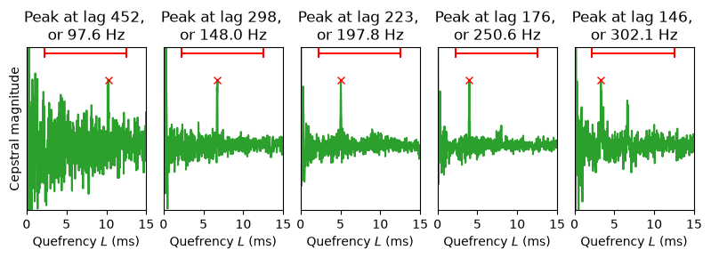
Source
print(f"Cepstrum: {mae_cents(fs/max_cepstral_peak, tone_reference):.0f} cents MAE vs pYIN")
Cepstrum: 5 cents MAE vs pYIN
The peaks are much more pronounced here in the cepstrum in the sense that they are sharp and easily distinguishable from the noise. Still, the same danger of octave jumps persists in the lowest and highest tones, as there are other high peaks in the search range (red lines). However, since the peaks are now narrow, we cannot easily interpolate between points to find a more accurate location of the peak.
Pitch contours and -tracking
Pitch is used in speech for expressive purposes. In particular, relatively high pitch (and intensity) segments typically indicate an emphasis. It is therefore important to observe changes in pitch over time. Such pitch-over-time plots are known as pitch contours. The challenge of finding “good” pitch contours, that avoids intermittent octave-jumps, is known as pitch tracking.
Here is a sample sentence that can be used to demonstrate pitch contours and -tracking.
Source
# Initialization
import matplotlib.pyplot as plt
from scipy.io import wavfile
import scipy
import scipy.fft
import numpy as np
import IPython
import librosa

filename = 'sounds/f0speechsample.wav'

#plt.rcParams.update({
#    "text.usetex": True,
#    "font.family": "Helvetica"
#})

# read from storage
fs, data = wavfile.read(filename)
datalength = len(data)
time = np.arange(datalength)/fs

IPython.display.display(IPython.display.Audio(data,rate=fs))
plt.figure(figsize=(6,3))
plt.plot(time,data)
plt.xlabel('Time (s)')
plt.ylabel('Amplitude')
plt.yticks([])
plt.show()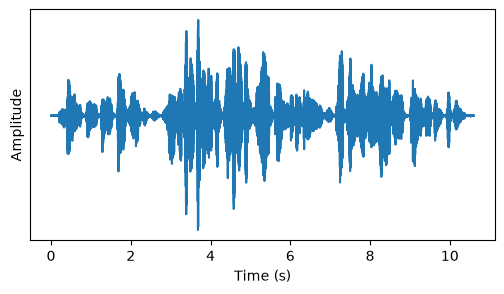
Source
window_step = window_length // 2
window_count = (datalength - window_length)//window_step - 1

f0estimates = np.zeros([window_count, 4])

f0pyin, voiced_flag, voiced_prob = librosa.pyin(data.astype(float),
                                    sr = fs, # sampling frequency
                                    fmin=f0_range_Hz[0],
                                    fmax=f0_range_Hz[1],
                                    frame_length=window_length,
                                    hop_length=window_step)

f0estimates[:,3] = f0pyin[1:window_count+1]

for window_ix in range(window_count):
    window = data[(window_ix*window_step):(window_ix*window_step+window_length)] * windowing_function

    correlation = np.correlate(window,window,mode='full')[window_length-1:]
    power_spectrum = np.abs(scipy.fft.rfft(window,n=fft_length))**2
    cepstrum = scipy.fft.irfft(10*np.log10(power_spectrum))

    max_corr_index = np.argmax(correlation[f0_range[0]:f0_range[1]])+f0_range[0]
    max_frequency_index = np.argmax(
        power_spectrum[f0_range_fft_indices[0]:f0_range_fft_indices[1]]) +f0_range_fft_indices[0]
    max_cepstral_index = np.argmax(cepstrum[f0_range[0]:f0_range[1]])+f0_range[0]

    f0estimates[window_ix, 0] = fs/max_corr_index
    f0estimates[window_ix, 1] = max_frequency_index*fs/fft_length
    f0estimates[window_ix, 2] = fs/max_cepstral_index
Source
plt.figure(figsize=(8,4))
t_axis = np.arange(0,window_count)*fs/(1000*window_step)
for i_col, label in enumerate(['Correlation','Spectrum','Cepstrum','pYIN']):
    plt.plot(t_axis, f0estimates[:,i_col], color=method_colors[label], label=label)
plt.legend(bbox_to_anchor=(1.01, 1.0))
plt.title('Pitch contour estimates')
plt.xlabel('Time (s)')
plt.ylabel('Pitch (Hz)')
plt.show()
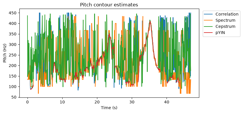
The figure illustrates four different estimates of the pitch contour; the above presented three methods as well as pYIN, which is an improvement of the classic YIN method De Cheveigné & Kawahara (2002)Mauch & Dixon (2014).
We can observe that near 35s, all four methods are nicely aligned, giving a continuous pitch contour. However, elsewhere, the three homebrew methods are very noisy. The first obvious reason is that the presented methods estimate a pitch in all frames, also when no voiced signal is present. We can use voice activity detection to limit analysis to only speech frames. This still leaves unvoiced frames for which we need some additional detection. We can, for example, check whether the detected peak is “prominent” or large enough in its surroundings such that it really is a peak and not noise. Also, if the detected maximum is at the border of the analysis range, that often indicates an anomaly, e.g. the maximum is likely outside the analysis range. Such heuristics should then be carefully tuned.
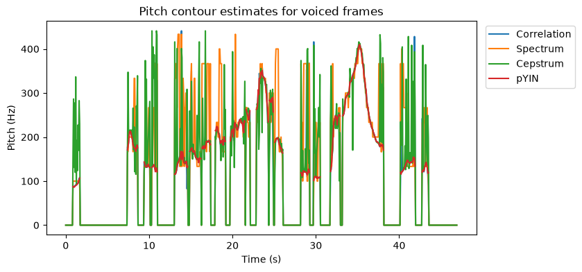
The pYIN library function used here (from Librosa) provides such a measure of voicing activity. By filtering the pitch contours to include only voiced frames, we obtain the following.
Source
plt.figure(figsize=(8,4))
t_axis = np.arange(0,window_count)*fs/(1000*window_step)
voiced = voiced_flag[1:window_count+1].astype(int)
for i_col, label in enumerate(['Correlation','Spectrum','Cepstrum','pYIN']):
    plt.plot(t_axis, f0estimates[:,i_col]*voiced, color=method_colors[label], label=label)
plt.legend(bbox_to_anchor=(1.01, 1.0))
plt.title('Pitch contour estimates for voiced frames')
plt.xlabel('Time (s)')
plt.ylabel('Pitch (Hz)')
plt.show()
Source
voiced_mask = voiced_flag[1:window_count+1].astype(bool)
reference = f0estimates[:,3]

for label, col in zip(['Correlation','Spectrum','Cepstrum'], range(3)):
    print(f"{label}: {mae_cents(f0estimates[:,col], reference, voiced_mask):.0f} cents MAE vs pYIN (voiced frames)")
Correlation: 85 cents MAE vs pYIN (voiced frames)
Spectrum: 454 cents MAE vs pYIN (voiced frames)
Cepstrum: 402 cents MAE vs pYIN (voiced frames)
This seems vaguely better as a large portion of the noise has been omitted. A better visualization could be to compare the three first estimates with pYIN individually and with discrete points for each frame rather than a line.
Source
plt.figure(figsize=(8,6))
t_axis = np.arange(0,window_count)*fs/(1000*window_step)
voiced = voiced_flag[1:window_count+1].astype(int)

for k, label in enumerate(['Correlation','Spectrum','Cepstrum']):
    plt.subplot(311+k)
    plt.plot(t_axis, f0estimates[:,3]*voiced, color=method_colors['pYIN'], linewidth=2)
    plt.plot(t_axis, f0estimates[:,k]*voiced, 'x', color=method_colors[label], markersize=1)
    plt.ylabel('Pitch (Hz)')
    plt.title(f'{label} estimate of pitch contour')
    plt.legend(['pYIN', label], bbox_to_anchor=(1.01, 1.0))
plt.xlabel('Time (s)')
plt.tight_layout()
plt.show()
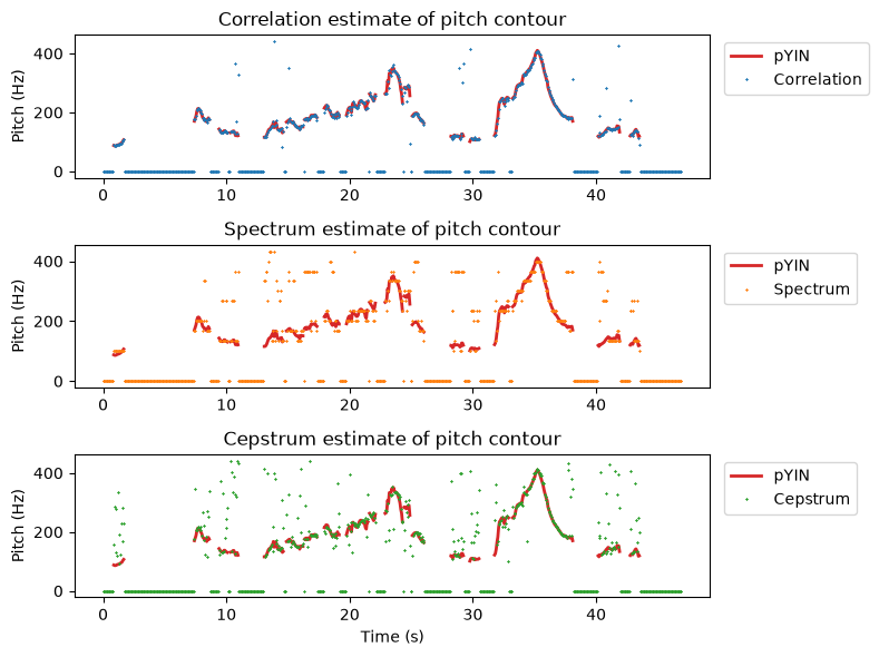
The (auto)correlation method clearly yields estimates which are closest to the high-quality estimates of pYIN, with a mean error of only about 85 cents -- a small fraction of a semitone -- over the voiced frames above. Estimates extracted from the power spectrum are quantized to discrete levels, which makes them less accurate even where they are otherwise correct, and they also feature many large errors, where often the estimate has clearly an octave error, such as at the very first segment where the red line is near 100 Hz, and some points are at the double frequency (an octave higher) near 200 Hz. These octave mistakes, each worth almost exactly 1200 cents, are frequent enough here (roughly one in ten voiced frames) that they dominate the average, giving the spectral estimate the largest mean error of the three methods, at around 450 cents.
The cepstral method has a smaller mean error, at around 400 cents, but this hides a different kind of problem: rather than clean octave jumps, most of its large errors are (seemingly) random values that do not correspond to simple multiples of the true pitch. This distinction matters for post-processing: octave errors can be fixed by checking whether the result could be a multiple of the true value and correcting when one is found, but that trick does not help with the cepstral method’s more haphazard mistakes. So despite its lower average error here, the cepstral method’s mistakes are the hardest of the three to remedy after the fact.
Neural estimators
More accurate and robust results can potentially be achieved by deep neural networks such as Crepe or DeepF0 Kim et al. (2018)Singh et al. (2021). Rather than picking peaks in a hand-crafted correlation, spectral, or cepstral domain, such networks are trained to map short frames of audio (or a time-frequency representation of them) directly to an estimate, learning the relevant feature extraction from data.
An openly available, actively maintained example of this approach is PENN (Pitch Estimating Neural Networks), a PyTorch toolkit for training and running neural pitch and periodicity estimators Morrison et al. (2023). Like the classical methods presented in this chapter, PENN estimates pitch independently for each short analysis frame and, alongside it, a periodicity score that serves as a voicing confidence. It then offers several ways of turning these per-frame estimates into a pitch contour: a simple per-frame argmax, a pYIN-style probabilistic threshold, or Viterbi decoding of the most likely path through the per-frame pitch likelihoods, the latter enforcing the kind of temporal continuity that our correlation, spectral, and cepstral estimates lacked. Its default pretrained model, FCNF0++, is trained across multiple datasets (e.g. MDB-stem-synth and PTDB) so as to generalise across recording conditions better than earlier, single-domain neural pitch trackers. PENN is thus a convenient, ready-to-use illustration of how such deep-learning-based estimators are packaged for practical use.
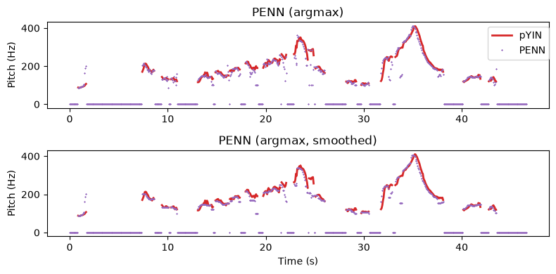
Let’s put PENN to the test on the same speech excerpt used above, and compare it with the classical estimators and pYIN.
Technical implementation details: PENN’s default decoder, Viterbi, relies on an optional companion package (
torbi) that ships precompiled binaries for specific torch/CUDA version combinations and has no fallback for unsupported ones; to keep this example reproducible regardless of the reader’s installed torch version, we instead use the'argmax'decoder, which — like our own correlation, spectral, and cepstral estimators — decides the pitch of each frame independently, without enforcing continuity with neighbouring frames.
Source
# Neural pitch estimation with PENN, using the audio already loaded above
# (`data`, `fs`) and the same hop size and frequency range as the classical
# estimators (`window_step`, `f0_range_Hz`). We avoid importing `torbi`
# (PENN's optional Viterbi-decoding backend, see above) so that this cell
# runs regardless of the reader's installed torch version.
import sys, types, logging, warnings
if 'torbi' not in sys.modules:
    sys.modules['torbi'] = types.ModuleType('torbi')
logging.getLogger('huggingface_hub').setLevel(logging.ERROR)
warnings.filterwarnings('ignore', category=FutureWarning)

import torch
import penn

audio = torch.tensor(data.astype(np.float32) / 32768.0).unsqueeze(0)

f0penn, periodicity_penn = penn.from_audio(
    audio,
    sample_rate=fs,
    hopsize=window_step/fs,
    fmin=float(f0_range_Hz[0]),
    fmax=float(f0_range_Hz[1]),
    decoder='argmax',
    gpu=None)

f0penn = f0penn.squeeze().numpy()
n_penn = min(window_count, len(f0penn))
Source
# A light median filter over a handful of frames, applied in the
# log-frequency (semitone) domain so that it treats octave errors
# symmetrically. This is a simple version of the idea proposed earlier in
# this chapter of comparing subsequent frames to curb octave jumps -- unlike
# PENN's own Viterbi decoder, it does not solve the underlying decoding
# problem, but it costs nothing beyond a few lines of numpy.
from scipy.signal import medfilt

smoothing_frames = 7
f0penn_smoothed = 2**medfilt(np.log2(f0penn), kernel_size=smoothing_frames)
Source
plt.figure(figsize=(8,4))
t_axis = np.arange(0,n_penn)*fs/(1000*window_step)
voiced = voiced_flag[1:n_penn+1].astype(int)

for k, (label, f0) in enumerate(
        [('PENN (argmax)', f0penn), ('PENN (argmax, smoothed)', f0penn_smoothed)]):
    plt.subplot(211+k)
    plt.plot(t_axis, f0estimates[:n_penn,3]*voiced, color=method_colors['pYIN'], linewidth=2)
    plt.plot(t_axis, f0*voiced, 'x', color=method_colors['PENN'], markersize=1)
    plt.ylabel('Pitch (Hz)')
    plt.title(label)
    if k==0:
        plt.legend(['pYIN','PENN'], bbox_to_anchor=(1.01, 1.0))
plt.xlabel('Time (s)')
plt.tight_layout()
plt.show()
Source
reference = f0estimates[:n_penn,3]                # pYIN, used as reference
voiced_mask = voiced_flag[1:n_penn+1].astype(bool)

print(f"Correlation:             {mae_cents(f0estimates[:n_penn,0], reference, voiced_mask):5.0f} cents MAE vs pYIN")
print(f"PENN (argmax):           {mae_cents(f0penn[:n_penn], reference, voiced_mask):5.0f} cents MAE vs pYIN")
print(f"PENN (argmax, smoothed): {mae_cents(f0penn_smoothed[:n_penn], reference, voiced_mask):5.0f} cents MAE vs pYIN")
Correlation:                85 cents MAE vs pYIN
PENN (argmax):             202 cents MAE vs pYIN
PENN (argmax, smoothed):   162 cents MAE vs pYIN
Despite FCNF0++ being, per frame, a considerably more accurate pitch model than our hand-crafted estimators, PENN’s argmax-decoded contour tracks pYIN worse than the simple autocorrelation estimator does (around 200 cents mean absolute error, versus about 85 cents for Correlation). The reason is decoding, not the network: pYIN’s own decoder (like PENN’s Viterbi and pYIN decoders) chooses the most likely path through consecutive frames, whereas 'argmax' commits to the best bin in each frame independently, in exactly the same frame-by-frame fashion as our Correlation, Spectrum, and Cepstrum estimators - and so it inherits the same vulnerability to octave errors and other isolated mistakes. Applying the light median filter above narrows the gap (down to roughly 160 cents at a 7-frame window) but does not close it, since a fixed-length filter is a crude substitute for the dynamic-programming search a real Viterbi decoder performs. This is a useful reminder that a neural network’s raw per-frame predictions are only part of the estimator; the decoding strategy that turns those predictions into a pitch contour matters just as much, for neural and classical estimators alike.
Discussion
Analysis of fundamental frequency often makes sense as it is a prominent feature of speech and has an expressive function. Classical DSP methods yield good results, though octave errors will always mar estimation. Here, we presented examples only with clean voices without background noises or reverberation. More realistic scenarios, that include background noise and competing speakers, obviously bring more problems.
Neural estimators such as those presented above can improve on these classical methods, provided their decoder makes proper use of the continuity between neighbouring frames, as our own PENN example illustrated. Beyond decoding, a data-driven approach brings its own challenge, namely to define the ground truth used for training. What is the true pitch? Who defines it and how is it determined? The ground truth is required by most data-driven approaches, yet both manual and automatic pitch estimation are susceptible to errors. The danger is that the model then approximates the method which was used to create the ground-truth, rather than the underlying phenomenon.
References
- De Cheveigné, A., & Kawahara, H. (2002). YIN, a fundamental frequency estimator for speech and music. The Journal of the Acoustical Society of America, 111(4), 1917–1930. 10.1121/1.1458024
- Mauch, M., & Dixon, S. (2014). pYIN: A fundamental frequency estimator using probabilistic threshold distributions. 2014 Ieee International Conference on Acoustics, Speech and Signal Processing (Icassp), 659–663. 10.1109/ICASSP.2014.6853678
- Kim, J. W., Salamon, J., Li, P., & Bello, J. P. (2018). Crepe: A convolutional representation for pitch estimation. 2018 IEEE International Conference on Acoustics, Speech and Signal Processing (ICASSP), 161–165. 10.1109/ICASSP.2018.8461329
- Singh, S., Wang, R., & Qiu, Y. (2021). DeepF0: End-to-end fundamental frequency estimation for music and speech signals. ICASSP 2021-2021 IEEE International Conference on Acoustics, Speech and Signal Processing (ICASSP), 61–65. 10.1109/ICASSP39728.2021.9414050
- Morrison, M., Hsieh, C., Pruyne, N., & Pardo, B. (2023). Cross-domain neural pitch and periodicity estimation. arXiv Preprint arXiv:2301.12258. 10.48550/arXiv.2301.12258