Modified discrete cosine transform (MDCT) - Introduction to Speech Processing

Introduction¶

In processing speech and audio, we often need to split the signal into segments or windows, because

audio signals are relatively slowly changing over time, such that by segmenting the signal in short windows allows assuming that the signal is stationary, which is a pre-requisite of many efficient methods such as spectral analysis,
transform-domain analysis, such as spectral analysis, requires that we transform the entire signal in one operation, which in turn requires that we have received the entire signal, before we can start processing. In for example telecommunications, this would mean that we have to wait for a sentence to finish before we can begin sending, and thus reconstruction the sentence at the receiver would have to wait until the whole sentence has finished, incurring a significant delay in communication.

In practical scenarios, we thus always apply windowing before processing.

Applying spectral processing, such as processing in the STFT domain, in telecommunications applications however has a significant drawback. We need windows which are overlapping to allow perfect reconstruction, that is, we require that we can perfectly reconstruct the original signal from the windowed signal. Overlaps however mean that consecutive windows share information from the same samples (see Figure on the right). The same information thus has to be encoded in both windows, which is inefficient. With coding a signal, our target is to compress the information to the fewest possible bits, but if we encode a part of the information twice, we increase the amount of information we need to encode. The STFT domain thus causes over-coding, where in effect, two different bit-streams could represent the same output signal.

The modified discrete cosine transform (MDCT) is a solution to the over-coding problem, which uses projection-operators at the overlaps such that the information in consecutive windows are orthogonal to each other. Since information is therefore perfectly retained, the amount of information is not increased nor decreased, and we say that this operator is critically sampled.

The MDCT thus provides a time-frequency representation of the input signal, where we can analyse and process the time-evolution of frequency-components. It shares most of the beneficial properties of the STFT, wherein a signal processed in the MDCT-domain, remains continuous in the time-domain and we can use FFT-based operations for efficient implementations. Perhaps the most significant difference between the STFT and MDCT, other than perfect sampling of the MDCT, is that where the STFT is a complex-valued representation, the MDCT is a real-valued representation when the input is real-valued.

Due to these beneficial properties of the MDCT, it is the most commonly used time-frequency transform in speech and audio coding and employed in standardized codecs such as MPEG USAC, 3GPP EVS and Bluetooth LC3.

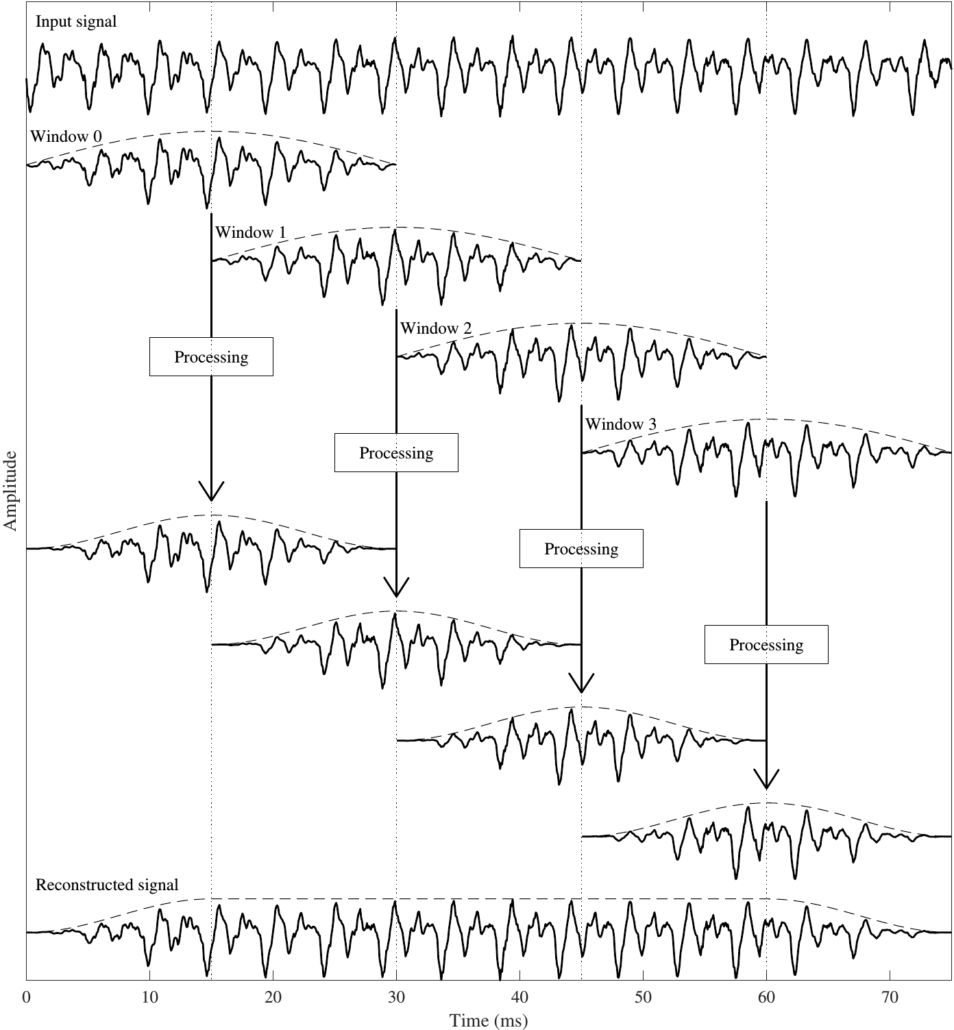
Executive summary of algorithm¶

The MDCT is based on taking the symmetric and anti-symmetric parts of the signal at the overlap, such that the symmetric part goes to the one window and the antisymmetric to the other. We furthermore window those symmetric and antisymmetric parts such that they converge smoothly to zero at the borders. Consecutive windows are thus orthogonal at the overlap such that information is split exactly in half and we obtain perfect reconstruction and critical sampling. Moreover, since the segments are windowed, we do not have any difficulties with discontinuities.

Secondly, we take the discrete cosine transform (DCT) of the windowed signal (=of the orthogonal projection). The conventional DCT has to, however, be adjusted such that its phase and symmetries match with the symmetric and anti-symmetric parts. Hence the name modified DCT or MDCT. The matching of symmetries is possible only through this modification of the DCT and cannot be generalized to the discrete Fourier transform (DFT).

The (anti)symmetric part of signal then “looks like the signal” which would have this symmetry. In other words, we introduce a deviation from the original signal and this deviation is known as a time-domain aliasing component, since it is similar to the aliasing effects which occur with the DFT. However, in reconstruction, we add the symmetric and anti-symmetric parts together, such that they cancel each other, which is known as time-domain aliasing cancellation (TDAC). The TDAC is equivalent with the orthogonal projection laying at the basis of the MDCT, and thus a central property of the MDCT.

Visual Explanation¶

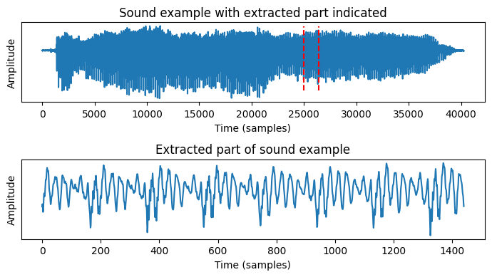
We start with a sound sample and extract a segment from it.

import matplotlib.pyplot as plt
import numpy as np
import scipy
import IPython.display as ipd 

sample_rate, data = scipy.io.wavfile.read('sounds/soundexample.wav')

window_length_ms = 30
window_length = (sample_rate*window_length_ms)//1000
window_step = window_length//2
window_count = 5

ix = np.arange(25000,25000+window_step*(window_count+1))

plt.figure(figsize=(7,4))

plt.subplot(211)
plt.title('Sound example with extracted part indicated')
plt.plot(data)
plt.plot([ix[0],ix[0]],[-10000,6000],'r--')
plt.plot([ix[-1],ix[-1]],[-10000,6000],'r--')
plt.ylabel('Amplitude')
plt.xlabel('Time (samples)')
plt.yticks([])

plt.subplot(212)
plt.title('Extracted part of sound example')
plt.plot(data[ix])
plt.xlabel('Time (samples)')
plt.ylabel('Amplitude')
plt.yticks([])

plt.tight_layout()
plt.show()

ipd.display(ipd.Audio(data,rate=sample_rate))

data = data[ix]

We can window this segment it with rectangular windows (i.e. no windowing function). The overlapping areas between windows are the regions between black dashed lines.

plt.figure(figsize=(7,4))
plt.plot(data)
for win_idx in np.arange(window_count,dtype=np.int32):
    start_idx = window_step*win_idx
    end_idx = start_idx + window_length
    idx = np.arange(start_idx,end_idx,dtype = np.int32)
    plt.plot(idx, data[idx]-12000*(win_idx+1))

for win_idx in np.arange(1,window_count+1):
    plt.plot(win_idx*window_step*np.array([1,1]),[8000, -12000*(window_count+.6)],'k--')

plt.ylabel('Amplitude')
plt.xlabel('Time (samples)')
plt.title('Windows with overlapping areas indicated')
plt.yticks([])
plt.tight_layout()

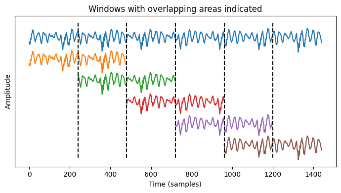
By definition, the same signal appears in every pair of subsequent windows. In transmission applications this is a problem, because the same information would then have to be transmitted twice.

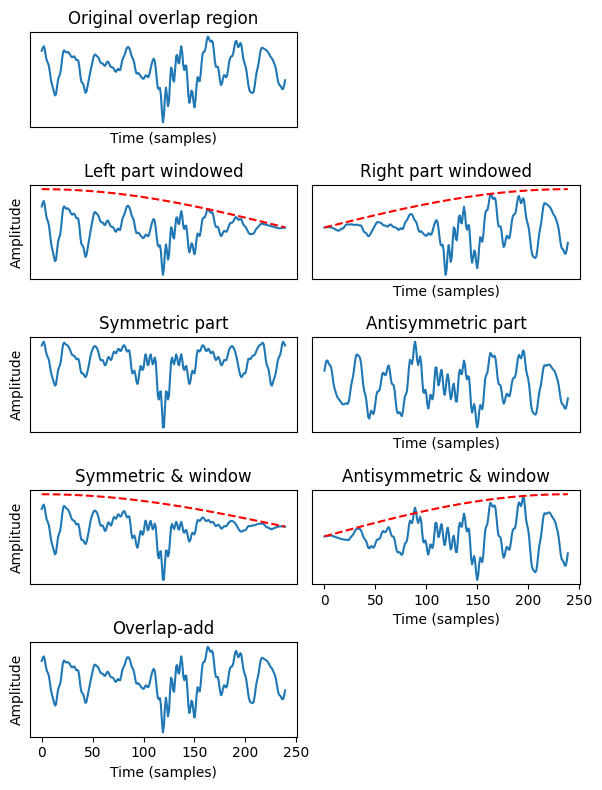
Such overcoding can be avoided by splitting the signal into two orthogonal parts in the overlaps. We can do this by splitting the signal into its symmetric and antisymmetric parts. The sum of the two parts then still adds up to the original signal.

plt.figure(figsize=(7,5))
plt.plot(data)

def Psplit(x):
    return .5*(x+np.flipud(x)), .5*(x-np.flipud(x))

for win_idx in np.arange(1,window_count):
    start_idx = window_step*win_idx
    end_idx = start_idx + window_step
    idx = np.arange(start_idx,end_idx,dtype = np.int32)
    s,a = Psplit(data[idx])
    plt.plot(idx, s-12000*(win_idx))
    plt.plot(idx, a-12000*(win_idx+1))
    plt.plot(idx, a+s -12000*(window_count+1),'k')

for win_idx in np.arange(1,window_count+1):
    plt.plot(win_idx*window_step*np.array([1,1]),[8000, -12000*(window_count+1.6)],'k--')

plt.ylabel('Amplitude')
plt.xlabel('Time (samples)')
plt.title('Windows with overlapping areas indicated')
plt.yticks([])

plt.text(-250,0,'Original')
plt.text(-250,-12000*(window_count+1),'Sum')
plt.tight_layout()

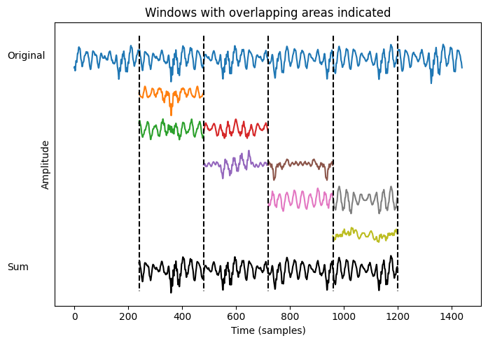
This split does not use any windowing function and thus we see that there are sometimes big discontinuities at the center of the window. Similar discontinuities will happen also at window edges, if the windows are modified befor reconstruction.

Surprisingly, this split into parts can be directly combined with windowing, before and after processing. The perfect reconstruction of the signal still works.

lwin = np.cos(np.pi*np.arange(.5,window_step)/(2*window_step))
rwin = np.flipud(lwin)

datawin = data[window_step:2*window_step]

plt.figure(figsize=(6,8))
plt.subplot(521)
plt.plot(datawin)
plt.xlabel('Time (samples)')
plt.title('Original overlap region')
plt.yticks([])
plt.xticks([])

plt.subplot(523)
plt.plot(datawin*lwin)
plt.plot(lwin*np.max(datawin),'r--')
plt.ylabel('Amplitude')
plt.title('Left part windowed')
plt.yticks([])
plt.xticks([])

plt.subplot(524)
plt.plot(datawin*rwin)
plt.plot(rwin*np.max(datawin),'r--')
plt.xlabel('Time (samples)')
plt.title('Right part windowed')
plt.yticks([])
plt.xticks([])

plt.subplot(525)
plt.plot(datawin*lwin + np.flipud(datawin*lwin))
plt.ylabel('Amplitude')
plt.title('Symmetric part')
plt.yticks([])
plt.xticks([])

plt.subplot(526)
plt.plot(datawin*rwin - np.flipud(datawin*rwin))
plt.xlabel('Time (samples)')
plt.title('Antisymmetric part')
plt.yticks([])
plt.xticks([])

plt.subplot(527)
plt.plot(lwin*(datawin*lwin + np.flipud(datawin*lwin)))
plt.plot(lwin*np.max(datawin),'r--')
plt.ylabel('Amplitude')
plt.title('Symmetric & window')
plt.yticks([])
plt.xticks([])

plt.subplot(528)
plt.plot(rwin*(datawin*rwin - np.flipud(datawin*rwin)))
plt.plot(rwin*np.max(datawin),'r--')
plt.xlabel('Time (samples)')
plt.title('Antisymmetric & window')
plt.yticks([])

plt.subplot(529)
plt.plot(lwin*(datawin*lwin + np.flipud(datawin*lwin)) + rwin*(datawin*rwin - np.flipud(datawin*rwin)))
plt.ylabel('Amplitude')
plt.xlabel('Time (samples)')
plt.title('Overlap-add')
plt.yticks([])

plt.tight_layout()
plt.show()

When applying the same process for all windows, we can reconstruct the whole signal.

hwin = np.cos(np.pi*np.arange(.5,window_step)/(2*window_step))

plt.figure(figsize=(7,5))
plt.plot(data)

def winsplit(x,hwin):
    fwin = np.flipud(hwin)
    l = hwin*x
    r = fwin*x
    return (l+np.flipud(l)), (r-np.flipud(r))

def winmerge(s,a,hwin):
    fwin = np.flipud(hwin)
    return s*hwin + a*fwin

for win_idx in np.arange(1,window_count):
    start_idx = window_step*win_idx
    end_idx = start_idx + window_step
    idx = np.arange(start_idx,end_idx,dtype = np.int32)
    s,a = winsplit(data[idx],hwin)
    plt.plot(idx, s-12000*(win_idx))
    plt.plot(idx, a-12000*(win_idx+1))
    plt.plot(idx, winmerge(s,a,hwin) -12000*(window_count+1),'k')

for win_idx in np.arange(1,window_count+1):
    plt.plot(win_idx*window_step*np.array([1,1]),[8000, -12000*(window_count+1.6)],'k--')

plt.ylabel('Amplitude')
plt.xlabel('Time (samples)')
plt.title('Windows with orthogonal overlap areas')
plt.yticks([])

plt.text(-310,0,'Original')
plt.text(-310,-12000*(window_count+1),'Overlap-add')
plt.tight_layout()

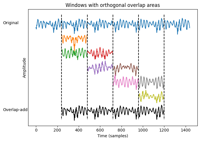
This representation is compatible with the discrete cosine transform (DCT), such that we can take the DCT of each window with orthogonal overlaps. We then obtain a time-frequency representation of the signal, where each frame is independent of all other frames.

Mathematical Definition¶

Suppose $x$ is a $N\times1$ vector representing the overlapping region shared by two consecutive windows, such as the are between 15 and 30 ms in the figure above and right. Our task is to design a projection matrix $P$ of size $N\times N$ , such that we can split $x$ into two orthogonal parts as

\begin{cases} x_L &= Px\\ x_R &= P_0x \end{cases}

(1)

where the $P_{0}$ is the kernel of $P$ and thus $P_0 P^T = 0,$ such that we can reconstruct $x$ as

P^T x_L+P_0^Tx_R = P^T P x + P_0^T P_0 x = (P^T P + P_0^T P_0)x = x,

(2)

since $P^T P + P_0^T P_0 = I$ by definition.

The vectors $x_{L}$ and $x_{R},$ corresponding to the left and right windows, are thus both of length N/2 and contain each exactly half the information of $x$ .

Though this is a mathematically clean solution, it is not practical, since after processing the reconstructed signal could have discontinuities. For example, suppose that we define $P$ as the operator which extracts the symmetric part of $x$ , that is, $P = [I, J]\sqrt{1/2},$ where $I$ is the $(N/2)\times(N/2)$ identity matrix and $J$ its left-right flipped counterpart (reverse diagonal). The kernel is then $P_0 = [I, -J]\sqrt{1/2}.$ If we make a small modification to the signal as $x_L':=x_L+d,$ then the reconstruction is $x':=P^Tx_L+P^Td+P_0^Tx_R=x+P^Td,$ which means that original signal is changed by $P^Td$ . Unfortunately, however, this component does not go to zero at the border such that processed signal is not continuous. Specifically, for example, consider a vector $d = [1,\,1,\,\dotsc,\,1]^T,$ which gives $P^Td = \sqrt{1/2}[1,\,1,\,\dotsc,\,1]^T,$ which is clearly non-zero at both ends of the vector.

The reason for this problem is that the definition did not include a windowing function. Recall that windowing is sample-by-sample multiplication of the signal with a windowing function. In matrix notation, we can implement this by multiplying the input signal $x$ with a diagonal matrix $W$ , where the diagonal elements correspond to the windowing function. The windowed signal is then $Wx$ . The symmetric projection $P$ can then be applied on the windowed signal such that the windowed left and right signals are

\begin{cases} x_L &= PWx := P'x\\ x_R &= P_0'x = P_0JWJx \end{cases}

(3)

where the $P_{0}'$ is the kernel of $P'$ , and $JWJ$ is simply the backwards part of the window (if $W$ is the increasing left part of the window, then $JWJ$ is the decreasing right part of the window). Note that the relationship between the two kernels, $P_0'=P_0JWJ$ applies only to the symmetric operator defined above, but generally not. In any case, the above definition now includes windowing and the orthonormal projection such that the beneficial properties of perfect reconstruction and critical sampling are retained, but now the signal is also going smoothly to zero at the edges, because we applied a windowing function.

Above we have thus developed a windowing operation which has the properties we need. However, our goal was to obtain a time-frequency transform of the signal, so we are still missing the time-frequency transform.

Our objective is to find a spectral representation of the windowed input signal. Importantly, note that above we studied the properties at the overlap, where we took an orthonormal projection of the overlap to obtain the left-part of the current window $x_{L}$ and right-part of the preceeding window $x_{R}$ . To avoid confusion, we here have to include the frame indices, such that the overlapping parts are now, respectively, $x_{L,k}$ and $x_{R,k-1}$ . The spectral representation, however, should come from a single frame, that is, we define frame $k$ as

\widehat x_k := \begin{bmatrix}x_{L,k} \ x_{R,k} \end{bmatrix}.

(4)

To obtain the spectrum of $\widehat x_k$ we can then multiply it with a time-frequency transform matrix $D$ , such that the frequency representation is $y_k=D\widehat x_k$ and the reconstruction is $\widehat x_k = D^T y_k,$ assuming that $D$ is orthogonal (as time-frequency transforms usually are).

In principle, the transform matrix $D$ could be any time-frequency transform (DFT, DCT-I, DCT-II, DST-I etc.), but we need to choose one specific. To evaluate the sanity of a particular choice, we should check how well the transform works together with the prior orthogonal projections. In particular, let us substitute the defitions of the left and right parts into the above equation to obtain

\widehat x_k := \begin{bmatrix}x_{L,k} \\ x_{R,k} \end{bmatrix} = \begin{bmatrix}PWx_k \\ P_0JWJx_{k+1} \end{bmatrix} = \begin{bmatrix}PW & P_0JWJ \end{bmatrix} \begin{bmatrix}x_k \\ x_{k+1} \end{bmatrix} := \hat P \begin{bmatrix}x_k \\ x_{k+1} \end{bmatrix}.

(5)

The combined windowing+projection+spectral transform is thus $y_k=D\hat P \begin{bmatrix}x_k \\ x_{k+1} \end{bmatrix} = M \begin{bmatrix}x_k \\ x_{k+1} \end{bmatrix}.$ To evaluate the sanity of a particular time-frequency transform, we thus have to study the basis functions of matrix $M$ . By exhaustively going through different options, it is simple to see that the implicit even/odd extensions of DCTs align with the symmetric/antisymmetric projections only for DCT-III. For the other options, we always get discontinuities in the basis functions.

Heuristically speaking, we want the basis functions to “look like” plausible signals, which could appear in a naturally appearing physical system. More formally, such “nice looking” basis functions have less leakage between spectral bins, and thus offer a more accurate description of the spectral characteristics of the input signal. Bäckström et al. (2017)

References¶

Bäckström, T., Lecomte, J., Fuchs, G., Disch, S., & Uhle, C. (2017). Speech coding: with code-excited linear prediction. Springer. 10.1007/978-3-319-50204-5