Glottal inverse filtering
Background
Speech signals can be roughly divided into three main categories according to their production mechanism (see e.g. Flanagan (1972) or Linguistic structure of speech). These three categories are
voiced sounds (e.g. [a], [n]), which are excited by the airflow signal generated by fluctuation of the vocal folds,
unvoiced sounds (e.g. [s], [f]), for which the sound excitation is turbulent noise, and
plosives (e.g. [k], [p]), which are transient-type sounds generated by abruptly releasing the air flow that has been blocked by the tongue or the lips.
From these three categories, we will focus in this section on voiced sounds. This group of speech sounds has been of special interest in speech research. because voiced sounds are more common than unvoiced sounds in many languages (in English, for example, 78% of speech sounds have been reported to be voiced Catford (1977).
Since vocal fold vibration and glottal excitation are key in production of speech, it is important have methodology to measure them. What makes a “good” voice? If the vocal folds are subject to a disruption, how does it affect the voice? This is often considered a medical question, but disruptions of voice have also large social and societal impacts. If your vocal folds do not function well, you cannot produce a proper glottal excitation and you might loose your voice. As a result of this, you can become isolated since you loose your ability to take part in speech communication. If you work in a voice-intensive profession such as in teaching, sales, singing or acting, also your ability to work relies on your voice. Therefore, disturbance in the voice impedes your ability to work. Studying the vocal folds and the glottal excitation it generates is therefore of great importance.
The excitation of voiced speech is the air flow that streams from the lungs and generates oscillations which take place in the mucosa (mucous membrane lining) of the vocal folds. This airflow excitation waveform is formally known as the glottal volume velocity waveform, but it is typically called shortly the glottal excitation. The word glottal comes from the orifice (i.e. opening) between the two vibrating vocal folds, the glottis (Figure 1).
The glottal excitation has an important role in speech communication because it is the acoustical source for most of the speech sounds that we use in our daily speech communication. Vibration of the vocal folds is quasi-periodic, that is, almost regular. This vibration results in a quasi-periodic structure of the glottal excitation, which in turn results in a quasi-periodic structure of the generated speech pressure signal. The vibration frequency of the vocal folds determines the fundamental frequency (F0) of the glottal excitation--and the F0 of the generated speech signal as well---and is therefore the source of pitch in speech. The vibration mode of the vocal folds is known as the phonation type which is varied by talkers when they change voice quality of their speech to sound, for example, breathy or pressed. For more information about analysis and utilization of voice source information, the reader is referred to the review article by Kadiri et al. (2021).
![Vocal folds (left), seen from above. The open space between the vocal
folds is called the glottis. By Henry Vandyke Carter - Henry Gray (1918) Anatomy of the Human Body (See “Book” section below)Bartleby.com: Gray’s Anatomy, Plate 956, Public Domain, (https://commons.wikimedia.org/w/index.php?curid=244424)[https://commons.wikimedia.org/w/index.php?curid=244424]](/build/Gray956-2e0c9b2464328470bace6438b1c6428c.png)
Figure 1:Vocal folds (left), seen from above. The open space between the vocal
folds is called the glottis. By Henry Vandyke Carter - Henry Gray (1918) Anatomy of the Human Body (See “Book” section below)Bartleby.com: Gray’s Anatomy, Plate 956, Public Domain, (https://
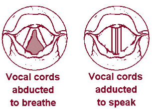
Figure 2:The glottis is open in the left panel and
closed in the right panel. By Henry Vandyke Carter - Henry Gray (1918) Anatomy of the Human Body (See “Book” section below)Bartleby.com: Gray’s Anatomy, Plate 956, Public Domain, https://
The vocal folds are located in the neck, covered and surrounded by cartilages. Direct measurement of the vocal folds is therefore difficult. As an example, visual imaging of the vocal folds by inserting an image sensor into the mouth/nostrils is uncomfortable to say the least. Even when it is possible, it is an invasive measurement impeding normal production of speech and giving measurements a bias of an unknown size. Moreover, since the vocal folds oscillate with a fundamental frequency that can be several hundreds of Hz, high-speed video imaging is needed. As an example, if F0 is equal to 400 Hz, an imaging system with a frame rate of 4000 Hz is needed to get 10 images of the vocal folds per one fundamental cycle. While high-speed imaging systems are today readily available, they need a lot of light, which generates heat, which might damage sensitive tissues in the larynx. Imaging with other methods, X-rays or magnetic resonance imaging, generally have a slower frame rate and some imaging techniques (like X-rays) also generate harmful radiation (especially at high frame rates). The cartilage surrounding the vocal folds also prevents ultrasound measurements.
The most widely used direct measurement of the vocal folds is electroglottography (EGG) (for a review, see Herbst (2020)). EGG measures the time-varying impedance of the vocal folds using electrodes that are attached to the skin in the neck. EGG measures conductivity, which is dependent on the contact of the vocal folds when the glottis opens and closes. Thus, EGG gives information about the vocal fold contact area during a glottal cycle. However, this information is usually one-dimensional which limits the usability of the measurement. EGG signals are also sensitive to the placement of the electrodes. EGG signals are also unable to carry useful information in cases when there is no contact of the vocal folds which happens, for example, in production of soft speech.
Even though the direct measurement of the vocal folds is difficult, recording the acoustic output of the voice production mechanism, the speech signal, is easy. With a microphone, we can record the speech pressure signal emitted from the mouth, and try to deduce the glottal excitation from the speech sound. The procedure is minimally invasive, because we do not need to insert any sensors inside or onto the speaker’s body. The airflow through the glottis is closely related to the movements of the vocal folds; when the vocal folds are open, air can flow and when they are closed, airflow is stopped.
When the glottal excitation transmits from the vocal folds through the oral and nasal cavities, it is acoustically shaped by the vocal tract (for details, again, see Speech production and acoustic properties); some frequencies are emphasised and others attenuated. To estimate the glottal excitation, we therefore need to cancel the acoustic effect of the vocal tract. Recall that the effect of the vocal tract can be efficiently modelled by, for example, a linear predictive filter (by assuming that the speech production apparatus is a linear system). We can thus first estimate a filter to model the effect of the vocal tract and then cancel the effect of the vocal tract from speech by filtering the speech signal through the vocal tract inverse filter. This process to estimate the glottal excitation from speech pressure signal recorded by a microphone is known as glottal inverse filtering (GIF) Alku (2011).
Glottal inverse filtering methods
The estimation of the glottal excitation based on GIF has been studied since the 1950’s. The early studies used analog antiresonance circuits to cancel the effect of the vocal tract. Since the 1970s, digital signal processing has been used in the development of GIF methods. The developed technologies differ mainly in the way the vocal tract transfer function is estimated. Most methods are based on LP analysis, which assumes that the vocal tract transfer function can be approximated by an all-pole filter. A widely used LP-based GIF method is closed phase (CP) analysis Wong et al. (1979). It is based on computing the vocal tract transfer function with LP from speech samples in the closed phase of the glottal cycle when there is excitation through the vocal folds. Another popular GIF method is iterative adaptive inverse filtering (IAIF) Alku (1992). In this method, the average effect of the glottal source on the speech spectrum during the open phase and closed phase of the glottal cycle is first cancelled from speech after which the vocal tract is estimated with LP. Examples of more recent GIF methods based on different variants of LP analysis are the quasi-closed phase (QCP) analysis Airaksinen et al. (2014) and the quadratic programming (QPR) approach Airaksinen et al. (2016). GIF methods have also been developed based on the joint optimization of the source and filter Fu & Murphy (2006)Schleusing et al. (2013)Auvinen et al. (2014)Alzamendi & Schlotthauer (2017). In these methods, parametric artificial glottal source models are used to represent the glottal flow pulse or its derivative in a parametric form. Another approach for GIF is state-space modelling which is based on a concatenated tube model of the vocal tract and the Liljencrants-Fant model of the source Sahoo & Routray (2016). By optimizing the model using extended Kalman filtering, estimates of the glottal source and intermediate pressure values within the vocal tract are obtained. GIF methods have also been developed using a combination of causal (minimum phase) and anticausal (maximum phase) components of the speech signal Bozkurt et al. (2005)Drugman et al. (2011)Drugman et al. (2012). In these methods, the response of the vocal tract and the return phase of the glottal flow are considered as causal signals, and the open phase of the glottal flow is considered as an anticausal signal. These signals are separated by a mixed-phase decomposition using analysis synchronized with the time instants of glottal closure.
Speech-based biomarking of state of health
The main function of speech is to enable communication between people by transferring linguistic information between speakers. In addition to its linguistic content, the speech signal, however, includes plenty of other information. This information includes paralinguistic issues such as vocal emotions (e.g. angry/sad/happy speech) and speaker traits (e.g. gender, age, height etc. of the speaker). One research topic that belongs to the latter category is biomarking the speaker’s state of health using his or her speech signal. As an example, the goal of biomarking could be to detect from speech whether the speaker has Covid-19 or not. This topic calls for signal processing and machine learning methodologies and has become an area of increasing interest in speech technology. The major issues underpinning this research topic will be shortly described in this section.
Benefits of the speech-based biomarking technology
The speech-based biomarking of state of health should not be seen as a technology to replace the true clinical diagnosis and care of patients. However, the speech-based biomarking of human health has a few benefits, which make it a justified topic of health and wellbeing technology. First, the input signal to the biomarking system, the speech microphone signal, can be recorded non-invasively in a comfortable manner using a cost-effective devise (e.g. phone). Second, the speech-based biomarking can be conducted outside hospital using a system that is easy to administer and can be used by the patient at home, thereby avoiding frequent and often inconvenient visits to the clinic. This is particularly useful, for example, for neurodegenerative diseases such as Parkinson’s disease and Alzheimer’s disease for which the speech-based biomarking can be used, in principle, in the early detection of the disease from telephone speech recordings. Even though the speech-based biomarking does not replace clinical examinations, it can be used in preventive healthcare technology to detect diseases at an early stage and to track physiological changes caused by the disease.
Machine learning tasks used in the study area
The most widely studied task in the topic is the detection task, that is, the binary classification problem in which speakers with a certain disorder (e.g. Parkinson’s disease, Covid-19 etc.) are distinguished automatically from healthy controls based on the recorded speech signals from both classes. In addition to the detection task, some investigations have addressed the biomarking topic from the multiclass classification’s point of view by studying, for example, 4-class classification where patients suffering from three known voice production disorders are classified from healthy talkers Chui et al. (2020). The severity assessment of the underlying disorder has also been studies as a regression problem, for example, related to Parkinson’s disease Bayestehtashk et al. (2015) and as a multi-class classification problem related to dysarthria Narendra & Alku (2021). Some studies have addressed progression of the underlying disorder using longitudinal analysis (e.g. Arias-Vergara et al. (2018)).
Technologies for the speech-based detection of disorders
Let us next take a closer look at the technologies that have been used in the detection task described above. The technologies developed can be roughly divided into two categories: (1) conventional pipeline systems and (2) modern end-to-end systems.
A detection system based on the conventional pipeline architecture consists of two separate parts: the feature extraction stage and the classifier stage (see Figure 3). In the former, the speech signal is expressed using a compressed set of selected acoustical features. In the latter, a machine learning model is used to distinguish speech features between the two classes (disordered vs. healthy). As shown in Figure 3, the detection system is data driven, that is, acoustical features are first extracted from speech signals labelled in a supervised manner (e.g. disordered vs. pathological) to train the classifier. By extracting the same acoustical features from test speech signals, a binary decision (i.e. disordered vs. healthy) can be made by the trained classifier for the input speech signal. A large number of different acoustical features have been used in the detection of disorders from speech. These features include classical, low-dimensional feature extraction methods such as mel-frequency cepstral coefficients (MFCCs) Davis & Mermelstein (1980) but also more high-dimensional features (such as openSMILE, Eyben et al. (2010)) consisting of tens of different individual parameters. In the classifier part of the classical pipeline system, many conventional machine learning classifiers have been used, particularly the support vector machine (SVM) has been widely used Kadiri & Alku (2020).
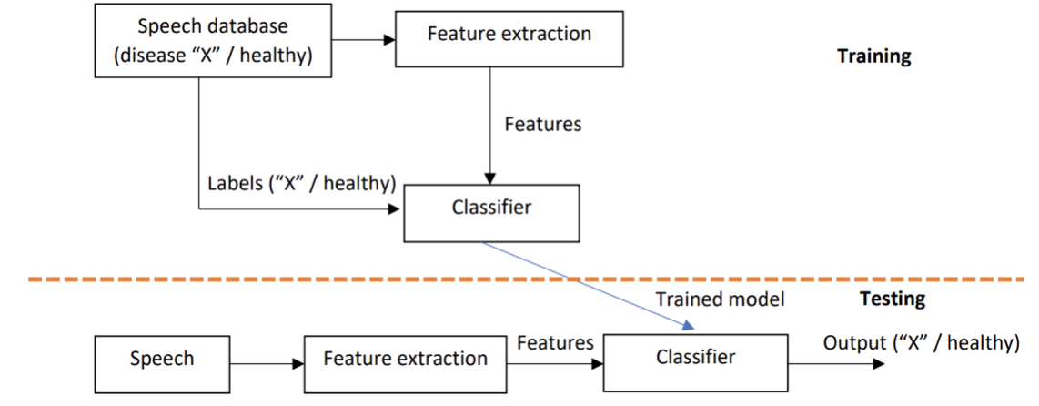
Figure 3:A general structure of a detection system based on the traditional pipeline approach. Speech database includes labelled speech signals (disease “X” vs. healthy). In the upper part, the classifier is trained using the labelled speech signals and selected features. In the lower part, the system is tested for an unseen speech signal. Classifier can be, for example, SVM.
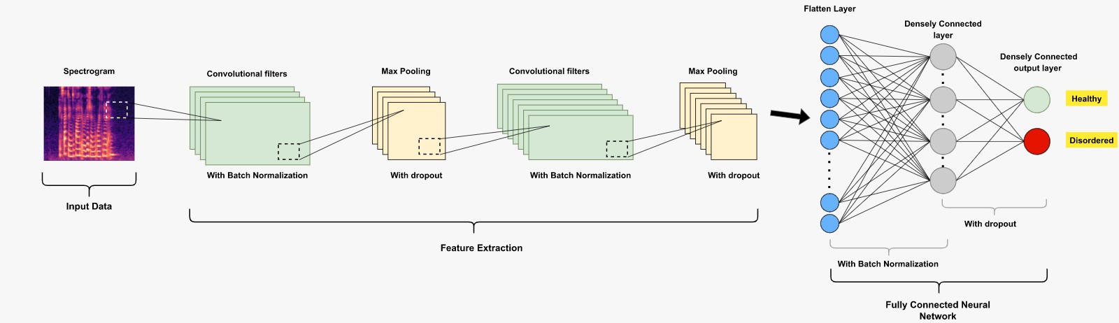
Figure 4:An example of a CNN-based deep learning classification system (healthy vs. disordered).
Classical pipeline systems have been increasingly replaced recently by end-to-end systems where the speech signal, expressed either as the raw time-domain signal (e.g. Millet & Zeghidour (2019)) or as the spectrogram (e.g. Vásquez-Correa et al. (2017)), is processed directly by deep learning methods to solve the underlying detection task. A block diagram describing an end-to-end system that uses spectrogram as input to the detection network is shown in Figure 4. As the deep learning architecture, most studies have used convolutional neural nets (CNNs). Some studies have also combined classical acoustic features--which are often referred to as hand-crafted features in this context--and deep-learned features (e.g. He & Cao (2018)). It is worth noting that deep learning -based end-to-end systems typically call for more training data than classical pipeline systems. Since the data in the topic area is recorded (partly) from patients, whose health condition might not enable long recordings, the amount of training data is typically limited in the study area. Therefore, classical pipeline systems are still a valid choice to build machine learning detection systems.
Disorders
Neurodegenerative diseases, particularly Parkinson’s disease and Alzheimer’s disease, are becoming prevalent globally due to aging of the populations. Parkinson’s disease has particularly been studied in the area of speech-based biomarking of human health (e.g. Arias-Vergara et al. (2018)Bayestehtashk et al. (2015)Vásquez-Correa et al. (2017)). In addition, neurodegenerative diseases such as Alzheimer’s disease (e.g. Warnita et al. (2018)) and ALS (e.g. Norel et al. (2018)) have been investigated in the study area. Other examples of disorders investigated are depression (e.g. Jiang et al. (2017)), voice production disorders (e.g. Garcı́a et al. (2019)) and sleep apnea (e.g. Botelho et al. (2019)). After the outbreak of Covid-19, many papers have addressed the detection of it either from speech or from voice signals such as coughs (e.g. Schuller et al. (2021)Sharma et al. (2022)).
Speech databases and speaking tasks
Studying biomarking of state of health involves using data-driven approaches where network parameters are trained using real speech produced by speakers affected by the underlying health problem. Publicly available databases exist for some diseases such as dysarthria (the TORGO database Rudzicz et al. (2012) and the UA Speech database Kim et al. (2008)), voice production disorders (the Saarbrucken voice database, SVD Pützer & Barry (2010)), and special language impairment Grill & Tučková (2016). Some of the open databases are, however, fairly small (e.g. with 10-20 speakers each producing a few utterances) which might limit the use of modern data-hungry deep learning networks. Speaking tasks are various, including simple repetitions of words, text reading and spontaneous speech. Some of the speaking tasks have been tailored to be more challenging to produce by the underlying patient population. An example is the diadochokinetic (DDK) task where the speaker is asked to repeat three-syllable units (i.e. /pa/-/ta/-/ka/). The DDK task is widely used in studying Parkinson’s disease Rusz et al. (2011).
- Flanagan, J. L. (1972). Speech Analysis Synthesis and Perception (2nd ed.). Springer-Verlag. 10.1007/978-3-662-00849-2
- Catford, J. C. (1977). Fundamental Problems in Phonetics (pp. 1–278). Indiana University Press.
- Kadiri, S. R., Alku, P., & Yegnanarayana, B. (2021). Extraction and Utilization of Excitation Information of Speech: A Review. Proceedings of the IEEE, 109(12), 1920–1941. 10.1109/JPROC.2021.3126493
- Herbst, C. T. (2020). Electroglottography – An Update. J. Voice, 34(4), 503–526. 10.1016/j.jvoice.2018.12.014
- Alku, P. (2011). Glottal inverse filtering analysis of human voice production-A review of estimation and parameterization methods of the glottal excitation and their applications. Sadhana, 36(5), 623–650. 10.1007/s12046-011-0041-5
- Wong, D. Y., Markel, J. D., & Augustine H. Gray, Jr. (1979). Least squares glottal inverse filtering from the acoustic speech waveform. IEEE Trans. Acoustics Speech Signal Process., 27(4), 350–355. 10.1109/TASSP.1979.1163260
- Alku, P. (1992). Glottal wave analysis with pitch synchronous iterative adaptive inverse filtering. Speech Communications, 11(2), 109–118. 10.1016/0167-6393(92)90005-R
- Airaksinen, M., Raitio, T., Story, B., & Alku, P. (2014). Quasi closed phase glottal inverse filtering analysis with weighted linear prediction. IEEE/ACM Trans. Audio Speech Lang. Process., 22(3), 596–607. 10.1109/TASLP.2013.2294585
- Airaksinen, M., Bäckström, T., & Alku, P. (2016). Quadratic programming approach to glottal inverse filtering by joint norm-1 and norm-2 optimization. IEEE/ACM Trans. Audio Speech Lang. Process., 25(5), 929–939. 10.1109/TASLP.2016.2620718
- Fu, Q., & Murphy, P. (2006). Robust glottal source estimation based on joint source-filter model optimization. IEEE Trans. on Audio Speech and Language Processing, 14, 492–501. 10.1109/TSA.2005.857807
- Schleusing, O., Kinnunen, T., Story, B. H., & Vesin, J.-M. (2013). Joint Source-Filter Optimization for Accurate Vocal Tract Estimation Using Differential Evolution. IEEE Trans. Audio Speech Lang. Process., 21(8), 1560–1572. 10.1109/TASL.2013.2255275
- Auvinen, H., Raitio, T., Airaksinen, M., Siltanen, S., Story, B. H., & Alku, P. (2014). Automatic glottal inverse filtering with the Markov chain Monte Carlo method. Comput. Speech Lang., 28(5), 1139–1155. 10.1016/j.csl.2013.09.004
- Alzamendi, G. A., & Schlotthauer, G. (2017). Modeling and joint estimation of glottal source and vocal tract filter by state-space methods. Biomed. Signal Process. Control, 37, 5–15. 10.1016/j.bspc.2016.12.022
- Sahoo, S., & Routray, A. (2016). A novel method of glottal inverse filtering. IEEE/ACM Trans. Audio Speech Lang. Process., 24(7), 1230–1241. 10.1109/TASLP.2016.2551864
- Bozkurt, B., Doval, B., d’Alessandro, C., & Dutoit, T. (2005). Zeros of z-transform representation with application to source-filter separation in speech. IEEE Sig.Pro. Letters, 12, 344–347. 10.1109/LSP.2005.843770